GSvit2D v 1.7

2D variant of GSvit is in a development phase and contains many untested algorithms. Its installed together with GSvit automatically and called the same way as 3D version, the only difference is that the parameter file must contain 2D dimensionality directive as a first item (to use this in 3D code is not mandatory, 3D dimensionality is a default option).

Calculation is performed for transversally electric (TE) mode or transversally magnetic (TM) mode depending on user request (parameter TMMODE).

Only subset of the algorithms provided for 3D is available now, due to fact that some methods are not working in 2D or are not yet implemented. Generally the parameter file is having very similar syntax to 3D version, however in some cases there are some small differences.

Note that we do not recommend using 2D code version for any production at this phase, it is still purely development part of GSvit software suite.

Parameter file description

Keywords are case sensitive. The following keywords can be used in the current version of GSvit (before issuing version 1.0 this means actual verison as obtained from SVN, but nearly all the parameters remain same for last issued binaries):

DIMENSIONALITY
2
Set the parameter file type to 2D computation. Note that in 3D version of GSvit you can use this directive as well (setting it to 3), but it is not obligatory.

POOL
xres yres dx dy
Set computation volume dimensions in pixels (xres, yres) and real pixel size - pixel spacing (dx, dy) in meters. To create a 200x200 pixel computational volume with pixel spacing of 1 micrometer, set:

COMP
nsteps
Set total number of computation steps, e.g. to set the number of steps to 100, write:

TMMODE
0/1
Set calculation mode to transversally electric (0) or transversally magnetic mode (1). This affects most of the algorithms as the unused field values for each particular mode are not calculated at all.

THREADS
nthreads
Set total number of threads to be used if we are calculating on CPU (not on GPU). Can be -1 for automated detection of number of cores and use of all of them which is also default behavior (since GSvit 1.3). Note that on systems using hyperthreading the virtual cores do not help (use half of available cores at maximum). Generally, FDTD is memory demanding and scaling with number of cores is therefore not linear (memory is the bottleneck), however up to some 8 threads there is significant speedup. You can test this scaling using ./gsvit test 3N, where N is problem size (e.g. 32 means thread test on 200x200x200 voxels). As and example, to set the number of threads to 4, write:

MEDIUM_LINEAR
filename
Use file that consists of binary data representing material, pixel by pixel. File structure is: xres, yres (binary 32-bit integers) of same size of computation volume, followed by four 2D fields of 32-bit floats representing epsilon, sigma, mu and magnetic conductivity. This approach is ideal for including complex or continuously varying geometries. For simple objects, use vector data input (MEDIUM_VECTOR), which is much simpler to construct.

MEDIUM_VECTOR
filename
Use file that consists vector material representation, composed from different basic entities (written in an ASCII file). Each entity entry is composed by the following information:

• type of entity (integer): 2 - circle, 3 - triangle, 4 - rectangle
• point coordinates in pixel values (doubles): x y z values for each point (single for circle, two for rectangle and three for triangle, plus eventually radius (for circle)
• material type (0: standard material, 1: tabulated material, 2: Drude model, 3: CP3 model 4: CP model, 10: perfect electric conductor, 99: data from optical database) followed by:
• relative permittivity, relative permeability, electric and magnetic conductivity as double values for material type=0, and 1 (both representing linear material)
• epsilon, omega_p and nu for type=2 (Drude model)
• epsilon, sigma and three sets of a, phi, omega and gamma for type=3 (CP3, in development)
• epsilon, omega, gamma and two sets of a, phi, omega and Gamma for type=4 (CP)
• nothing for material type=10 (PEC)
• material name for material type=99, e.g. Al2O3

so the entry looks for example as (4 100 100 20.5 0 22.13 1 0 0) for circle with radius 20.5 pixels, position (100, 100) and relative permittivity of 22.13 (rest or material properties is same as for vacuum).

Note that at present version of the 2D code the CP, CP3 model and Drude model is not implemented yet.

BOUNDARY_ALL
type
Set boundary condition of whole volume to a given type:

• none which means no boundary treatment providing reflection similar to perfect electric conductor,
• liao which means 2nd order absorbing (Liao) providing quite good absorption.

BOUNDARY_X0/BOUNDARY_XN/BOUNDARY_Y0/BOUNDARY_YN
type
Set boundary condition of a given boundary to a given type (types are same as for BOUNDARY_ALL). Field sources

SOURCE_POINT
i j mode (filename, values)
Point source at position (i j) using electric and magnetic field intensity time dependence described in file filename (mode=0) or generating such file for sine or pulsed sine waveform. If a text file is used, it consists of integer determining total number of values and succesive sets of values consisting of (step, ex, ey, ez, hx, hy, hz). For "mode=1" the source file is automatically generated (file "tmpsource" in the current directory) providing a sine wave source; the parameter after "mode" is therefore wavelength in meters followed by electric field amplitude. Finally, two parameters theta and phi determine the source orientation. For "mode=2" the same happens for sine wave damped by a gaussian envelope, parameter "mode" is therefore followed by wavelength and by gaussian envelope width, given in integer steps of the simulation (e.g. 20), and then electric field amplitude. Again, at the end, two parameters theta and phi determine the source orientation. Theta and phi equal to zero correspond to x-direction electric field point source.

Note that for generated source the orientation should match the mode of calculation (transversally electric or transversally magnetic. So for example setting

SOURCE_POINT
50 50 1 0.633e-6 1 0 0

fits to transversally magnetic mode, e.g.

TMMODE
1

Similarily to do a source for transversally electric calculation, write

and then

TMMODE
0

SOURCE_TSF
i_start j_start i_end j_end phi psi mode (filename, values)
Plane wave source using total/scattered field formulation. First four integers determine area that is used for field propagation, Phi determines wave direction and psi its polarisation. Parameter "mode" distincts different source definition. For "mode=0" a filename is provided pointing to a text file containing number of values N followed by N pairs of values step number - electric field value. N needs to be at least the total number of steps in simulation. For "mode=1" the source file is automatically generated (file "tmpsource" in the current directory) providing a sine wave source; the parameter after "mode" is therefore wavelength in meters followed by electric field amplitude. For "mode=2" the same happens for sine wave damped by a gaussian envelope, parameter "mode" is therefore followed by wavelength and by gaussian envelope width, given in integer steps of the simulation (e.g. 20), and then electric field amplitude.

Note that in present version the TSF source is in vacuum, material cannot cross it.

Orientation of axes of incoming wave comes from 3D version, assuming that theta=90 degrees. It is shown in the following image, table shows some typical useful values of parameters:

direction	polarisation	phi [deg]	psi [deg]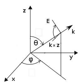
x axis	y	0	0
x axis	z	0	90
y axis	x	90	0
y axis	z	90	90

Note that TSF is not yet implemented on GPU.

Note that in present version every output needs GPU data to be synchronized with CPU, which can take significant time. For really fast simulations try to reduce frequency of data outputs.

OUT_FILE
filename.gwy
Set filename that will be used for outputing data. Gwyddion file (*.gwy) holds all data cross-sections (2d data).

OUT_POINT
Ex/Ey/Ez/Hx/Hy/Hz/All nskip i j filename
Output values of given component of electric/magnetic field into text file (filename).

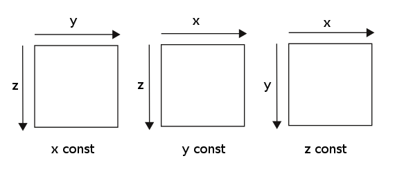
OUT_IMAGE
Ex/Ey/Ez/Hx/Hy/Hz/All/Epsilon/Sigma/Mu/Sigast nskip description
Output image of plane cross-section. Which plane is used is determined by indices i j k; two of them must be -1. All results are saved to a .gwy file, skipping given number of steps (e.g. not outputing image in every step unless nskip=1). Description is a string shown for the channel in Gwyddion data browser.

Note that Gwyddion shows data with top-left corner being center of coordinates, orientation of axes on what is seen in Gwyddion is show below (for 2D code we have always the z constant condition met, so axes are oriented as seen at the right image)

OUT_SUM
component skip i_start j_start k_start i_end j_end k_end epsilon mu sigma sigma* filename
Output sum of electric field intensity (components: ex, ey, ez, all) or absorption (component: abs) extracted from bounding box and material with given properties (epsilon only used for this). If epsilon is -1, no control of this parameter is done and whole box is used. Parameter "skip" controls frequency of file output only (and sync with GPU eventually), values are calculated at each time step anyway and will be output for intermediate steps as well. At present this is tested only on CPU.

GPU
ngpus
Set number of graphics cards to be used (indexed as CUDA indexes them). If this command is not used or set to zero, calculation is performed on PC processor. See example 1 for details of use. Note that at present version use of multiple GPUs together is implemented, but untested.

UGPU
number
Set GPU with given index to be used for calculations (indexed as CUDA indexes them). This can be used for example to run several different calculations on different cards. See example 1 for details of use.

VERBOSE

0-4

Set text output (step by step), from full (4) to silent mode (0).

Examples

Examples are in preparation. Check summary of some of tested parameter files for 2D problems.