Total/scattered field example

Summary

We will use cubic volume with Liao absorbing boundary condition and Total/scattered field plane wave source. Outputs cross-sections to a Gwyddion file and point values in three different locations in scattered field region to text files. A perfect electric conductor (PEC) sphere is located in the center.

What can be tested in this configuration:

• use of TSF source (try different angles for incident wave)
• PEC and other material conditions

Setup all this with XSvit

Note that some of the screenshots might be from an older version of XSvit.

First, start the XSvit application. If haven't done this before, setup the location of GSvit and Gwyddion under File->Preferences menu, so you can run the calculation from the GUI and see the results afterwards. Otherwise you will be able to use GUI only for parameter file setup. Many details concerning basic use of XSvit can be found in basic appplication use example. Here we will focus only on additional parameters settings.

First, we will set the basic parameters - computational space volume to 100x100x100 voxels and discretisation to 10 nm. We will compute 300 steps of the FDTD algorithm. This all can be set by double clicking on appropriate entries in the parameters list.

Now we will add a Total/Scattered Field source. This can be done using menu entry Edit parameters->Add TSF source. The dialogue shown below appears. We set the point source properties, i.e. volume where it is used in voxel coordinates, its type (load from file or construct a temporary file for it with sine wave or sine impulse) and orientation (see the angles for TSF in GSvit documentation). Note that for automatically generated sources like that one that we have used we should set the default directory (e.g. by saving or opening parameter file) before setting the source. Adding a TSF source will create a plane wave inside the volume.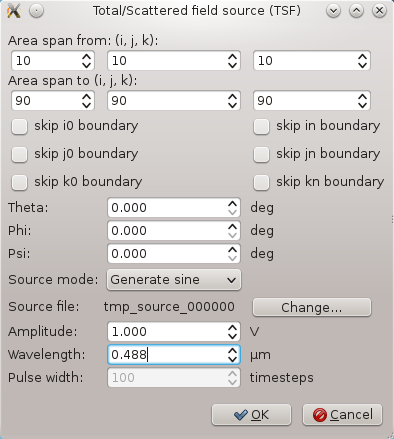

We will also add one image output for Ey component displayed in the yz plane.

After adding the source and outputs we can see it in the 3D window as shown below and also on the list of entries.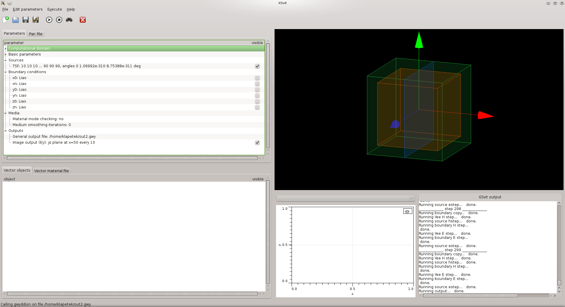

Finally, we will set the boundary conditions to absorbing (Liao) in order to prevent reflection of light scattered in the computational volume (in next part of the example, now there is nothing to scatter). Now we can save the parameter file and afterwards run the computation. Image output comes to general output file that can be opened by Gwyddion open source software via a menu command. We can see an undisturbed plane wave traveling across computational volume.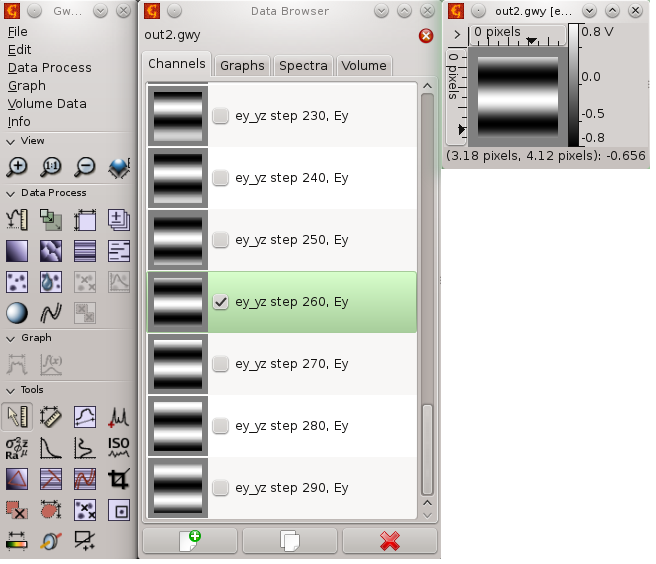

Now we can add some material into the computational volume, so we can see scattering of the plane wave. We will first add a perfect electric conductor sphere to the center. Use menu entry Edit material objects->Add sphere and setup a sphere with radius of 20 voxels, position 50,50,50 voxels and perfect electric conductor material. Sphere will be listed in vector objects entries. If you check the vector material file tab, you should see similar entry (you could write it directly as well):

4 50 50 50 20 10

Save this material file using File->Save material file as... into a file, here we have chosen filename smallsphere.txt. Then click on some of the entries in "Media" part of parameters and add file with this name

When you have look on "Vector objects tab" you can see already your sphere listed there. This is how it show look as (note that we have it listed under media parameters already).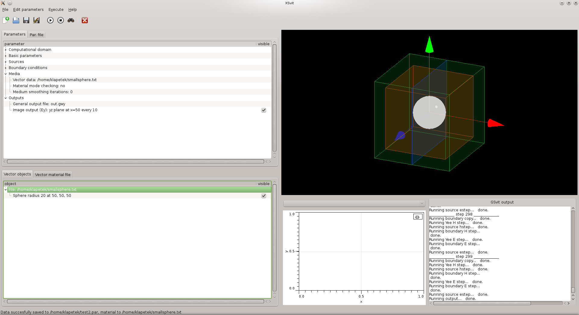

Now, when you hit "Save" button, bot the parameter file and media file is saved, as you can see on the status bar. You can run the computation and afterwards view the output, you should see something similar: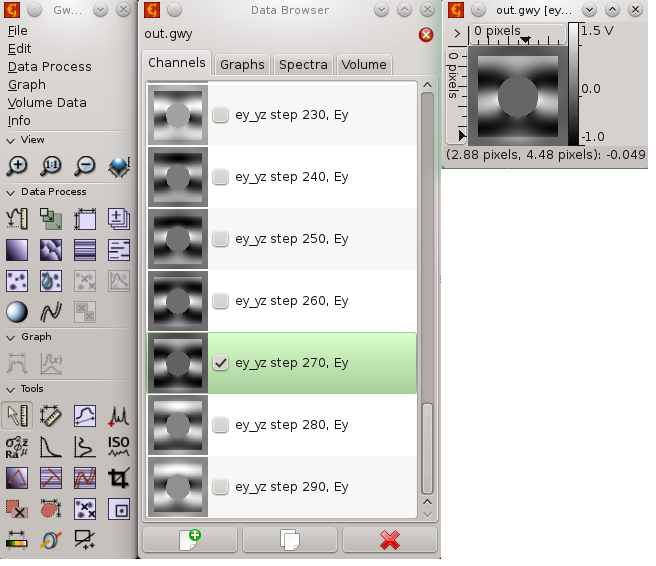

Let's use a different material of the sphere, e.g. with known dielectric properties. Double-click on sphere to edit it and and assign it to have voxel-by-voxel material properties with relative permittivity of 3, relative permeability 1 and zero losses. Alterinatively this can be done by modifying the material file directly to

4 50 50 50 20 0 3 1 0 0

Dielectric properties can be also loaded from database, again using GUI and assigning SiO2 database entry to material properties or writing this to vector material file:

which means that wavelength of the source will be analysed and appropriate dielectric properties for the selected material (here SiO2) will be used automatically. Result can be seen on the following output.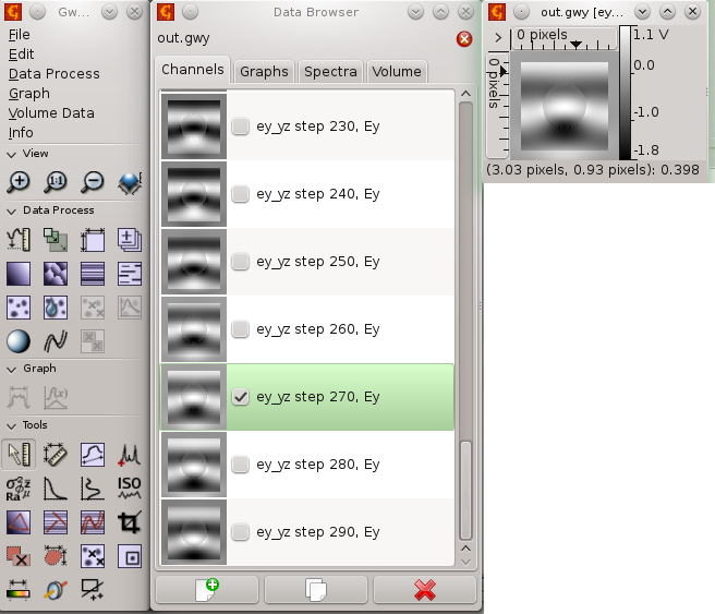

Download parameter file for this example: xex18_2.par

Next example

Back to the documentation.