|
News Features Documentation Download Participate |
Force acting on a non-spherical particleSummaryWe will setup cubic volume with a tetrahedral mesh based dielectric particle inside, absorbing boundary conditions, TSF source and we will evaluate optical scattering force acting on the particle. What can be tested:
Setup all this with XSvitNote that some of the screenshots might be from an older version of XSvit. Start the XSvit application and setup the computational volume in this way:
We refer to basic appplication use example for details how to adjust all these settings. Then we save the parameter file if we haven't done it before. We will first try to calculate optical force on a spherical particle, which is quite simple - we add a particle with radius 40 voxels to the center by writing 4 100 100 100 40 0 3 1 0 0 into vector material objects file, we save it using menu entry File->Save material file as... and we add the file to media entries in parameter list (by clicking on any of the Media items). Then we can add the force output by Edit->Add force output... which calls the following dialogue: 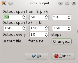
After setting all this the complete setup should look like this 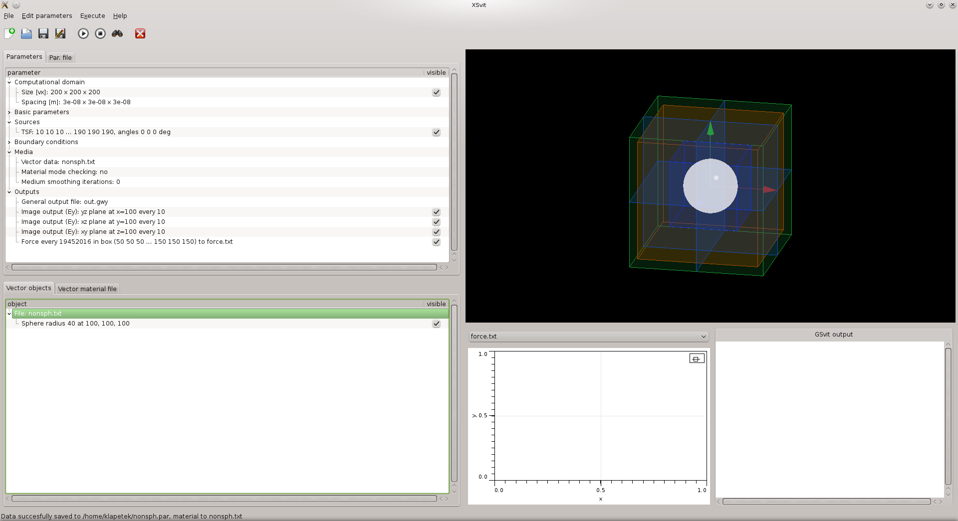
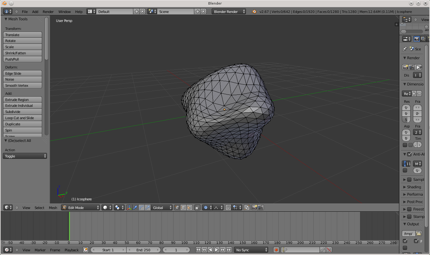
Then we can run the computation. Resulting force (in x, y, and z direction) is stored in the file. Total force can be also seen in the graph widget in XSvit. Now we can setup a tetrahedral mesh based non-spherical particle. Here we need to use an external application to create its geometry first. We will use Blender for this. There are many manuals available for Blender so we won't repeate them (and we are not experts on Blender modeling anyway), so there are just few points what we can do to create a particle:
Once we have tetrahedral mesh prepared, we can add this to vector material objects file. Remove spherical particle that we used before and write 21 particle.1 0 0 90 100 100 30 30 30 0 3 1 0 0This means adding mesh (type of object = 21), written in particle.1.ele and particle.1.node, using no material attributes, magnifying it by factor of 30,30,30 (in x,y,z direction) and shifting to 90, 100, 100. It will be filled with dielectric material with relative permittivity of 3. Note that particle needs to be within the force evaluation box. This is how it might look after setting it up: 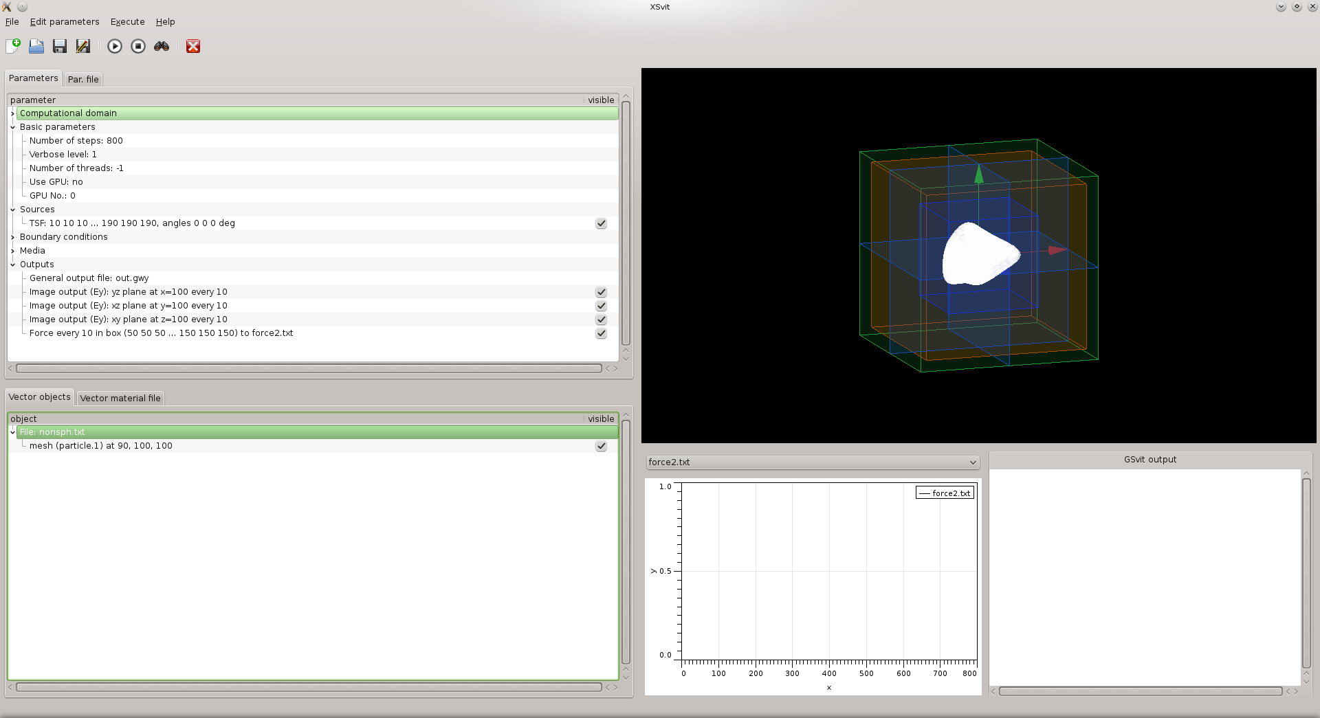
Now you can run the computation and evaluate plane wave interaction with your particle and evaluate scattering by this particle and optical force acting on it. The cross section output might look like this (depending on how exactly your particle looks like): 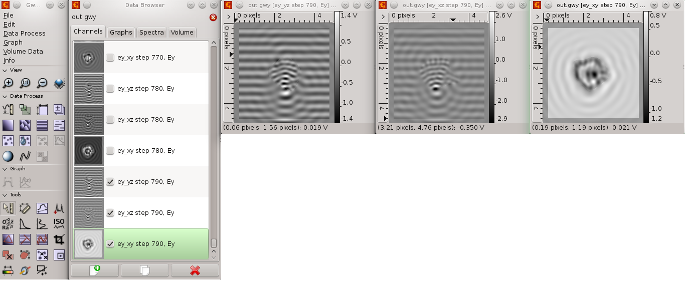
Output force graph is shown below. Note that as we typically want to know steady solution, we are interested in force at the right side of the graph and obviously we could have even more computation steps to let it be stable. In some cases, when some resonance modes should be developed within the particle, this can mean tens of thousands of time steps even. 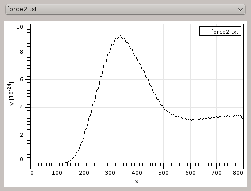
Here you can also download sample parameter file, material file and files particle.1.ele and particle.1.node (c) Petr Klapetek, 2013 |