GSvit v 1.5 and earlier

GSvit architecture is based on use of computational core (gsvit) and set of GUI front/backends for concrete applications (solar cell scattering, scanning near-field optical microscopy, etc.)

Note that meanwhile the core is already developed and tested for several years (now only being converted to software presented on these pages), the front/backends are still under development and will not be available soon.

Installation

Please see the download page.

Running the computational core

To run a regular calculation, GSvit program must be started with parameter file as a command line argument. If any other files are used (e.g. to specify material or source) these are also mentioned in the parameter file. Parameter file is an ASCII file composed by keywords and sets of values corresponding to these values. Rows can be commented out using '#' character at the beginning of the row. Check examples at end of this page to see some working parameter files.

Automated tests

If GSvit is started with "test" as an argument, followed by test number, it can run an automated test. For key tests even a precomputed value is installed, so result can be compared to it automatically. If a GPU is present in the computer and GSvit is translated with GPU support, it is recognized, reported and used for comparison to CPU.

Tests can be useful namely when installing GSvit on a new system or in doubts whether a concrete algorithm does not do what is expected.

Automated tests available are as follows (run gsvit with no arguments for a list of them):

• ./gsvit test 0 checks available GPUs only, printing their main characteristics.
• ./gsvit test 1 makes single test on CPU and all GPUs (if there are any)
• ./gsvit test 2 tests key algorithms performance, running approximately ten different tests for 100x100x100 voxels, 100 steps, which takes some ten minutes.
• ./gsvit test 3 tests key algorithms performance, running approximately ten different tests for 200x200x200 voxels, 300 steps, which can take tens of minutes, however is more precise regarding peak GSvit performance estimation.
• ./gsvit test 12 compares GPU/CPU time scaling up to 200x200x200 voxels
• ./gsvit test 13 compares GPU/CPU time scaling up to 300x300x300 voxels
• ./gsvit test 14 compares GPU/CPU time scaling up to 400x400x400 voxels
• ./gsvit test 15 compares GPU/CPU time scaling up to 500x500x500 voxels
• ./gsvit test 20 compares GPU time scaling up to 400x400x400 voxels
• ./gsvit test 3N tests multiple threads speedup on N00xN00xN00 voxels (i.e. 100 to 900 for 31 to 39)
• ./gsvit test AAABCDEF is a general test format. The eigth digit number AAABCDEF means:
  • AAA - cube size in pixels (i.e. if XXX = 100, cube size is 100 x 100 x 100)
  • B - boundary condition: 0 - none, 1 - PEC, 2 - Liao, 3 - CPML
  • C - material (small piece of it in the center of computational space): 0 - none, 1 - electric only, 2 - magnetic only, 3 - tabulated electric, 4 - tabulated magnetic, 5 - pec, 6 - Drude, 7 - CP
  • D - check material and appl optimum mode for saving some memory: 0 - no, 1 - yes
  • E - run Near-to Far Field transformation for a single point: 0 - no, 1 - yes
  • F - source: 0 - point source, 1 - total/scattered field, 2 - scattered field

The "AAABCDEF" naming is used also to store the precomputed data that are compared with tests results. The precomputed data for comparison are typically single near field or far field point time dependence.

There are two more tests designed for benchmarking HPC systems:

• ./gsvit benchmark N tests N threads computational time on 900x900x900 voxels
• ./gsvit bigbenchmark N tests N threads computational time on 4000x4000x4000 voxels

Parameter file description

Keywords are case sensitive. The following keywords can be used in the current version of GSvit (before issuing version 1.0 this means actual verison as obtained from SVN, but nearly all the parameters remain same for last issued binaries):

POOL
xres yres zres dx dy dz
Set computation volume dimensions in pixels (xres, yres, zres) and real pixel size - pixel spacing (dx, dy, dz) in meters. To create a 200x200x200 pixel computational volume with pixel spacing of 1 micrometer, set:

COMP
nsteps
Set total number of computation steps, e.g. to set the number of steps to 100, write:

THREADS
nthreads
Set total number of threads to be used if we are calculating on CPU (not on GPU). Can be -1 for automated detection of number of cores and use of all of them which is also default behavior (since GSvit 1.3). Note that on systems using hyperthreading the virtual cores do not help (use half of available cores at maximum). Generally, FDTD is memory demanding and scaling with number of cores is therefore not linear (memory is the bottleneck), however up to some 8 threads there is significant speedup. You can test this scaling using ./gsvit test 3N, where N is problem size (e.g. 32 means thread test on 200x200x200 voxels). As and example, to set the number of threads to 4, write:

MATMODE_CHECK
0/1
Check material settings and if possible, run computation with smaller memory allocation - not allocating some of the components and using simplified equations (e.g. for nonmagnetic materials or vacuum). This can save up to half computation time or memory requirements. A safe variant if something fails is 0 which is default value (full calculation). This might be necessary for some novel algorithms before they are tested properly, typically algorithms on GPU where this parameter is not recommended for now. An example of use is:

MEDIUM_LINEAR
filename
Use file that consists of binary data representing material, pixel by pixel. File structure is: xres, yres, zres (binary 32-bit integers) of same size of computation volume, followed by four 3D fields of 32-bit floats representing epsilon, sigma, mu and magnetic conductivity. This approach is ideal for including complex or continuously varying geometries. For simple objects, use vector data input (MEDIUM_VECTOR), which is much simpler to construct.

MEDIUM_VECTOR
filename
Use file that consists vector material representation, composed from different basic entities (written in an ASCII file). Each entity entry is composed by the following information:

• type of entity (integer): 4 - sphere, 7 - cylinder, 8 - parallelepiped, 12 - tetrahedron, 21 - tetrahedal mesh in Tetgen output format, 22 - Gwyddion height field
• point coordinates in pixel values (doubles): x y z values for each point (single for sphere, two for cylinder or parallelepiped and four for tetrahedron), eventually radius (for sphere and cylinder), or more complex entries (see below) for tetrahedral mesh or Gwyddion height field.
• material type (0: standard material, 1: tabulated material, 2: Drude model, 3: CP3 model 4: CP model, 10: perfect electric conductor, 99: data from optical database) followed by:
• relative permittivity, relative permeability, electric and magnetic conductivity as double values for material type=0, and 1 (both representing linear material)
• epsilon, omega_p and nu for type=2 (Drude model)
• epsilon, sigma and three sets of a, phi, omega and gamma for type=3 (CP3, in development)
• epsilon, omega, gamma and two sets of a, phi, omega and Gamma for type=4 (CP)
• nothing for material type=10 (PEC)
• material name for material type=99, e.g. Al2O3

so the entry looks for example as (4 100 100 100 20.5 0 22.13 1 0 0) for sphere with radius 20.5 pixels, position (100, 100, 100) and relative permittivity of 22.13 (rest or material properties is same as for vacuum). Material file for two dielectric nonabsorbing spheres and single absorbing parallelepiped can therefore look like:

4 50 100 100 20.5 0 22.13 1 0 0
4 150 100 100 20.5 0 22.13 1 0 0
8 30 30 160 170 170 170 0 20 1 2000 0

Note that the material data are interpreted succesively, overwriting previous values in the computational volume if there is an intersection, so you can create relatively complex geometries. Also, if there is MEDIUM_LINEAR, directive as well in the parameter file, this is performed before MEDIUM_VECTOR data interpretation (so vector data can overwrite them).

See Example 2 for more details of material parameters use.

For metals, CP model is at present the most suitable approach implemented in GSvit. CP model (in fact Drude + 2 critical points model) is based on this work: A. Vial, T. Laroche, Appl Phys B (2008) 93: 139-143, giving the following values for different materials (here already in GSvit material file format including material type (4)):

4 15.833 1.3861e16 4.5841e13 1.0171 -0.93935 6.6327e15 1.6666e15 15.797 1.8087 9.2726e17 2.3716e17 (silver)
4 1.1431 1.3202e16 1.0805e14 0.26698 -1.2371 3.8711e15 4.4642e14 3.0834 -1.0968 4.1684e15 2.3555e15 (gold)
4 1.0000 2.0598e16 2.2876e14 5.2306 -0.51202 2.2694e15 3.2867e14 5.2704 0.42503 2.4668e15 1.7731e15 (aluminium)
4 1.1297 8.8128e15 3.8828e14 33.086 -0.25722 1.7398e15 1.6329e15 1.6592 0.83533 3.7925e15 7.3567e14 (chromium)

If tetrahedral mesh is provided in Tetgen .node and .ele format, the following parameters are given after entity type (precending material type and material parameters):

Parameter filebase determines the filename of .node and .ele files (filebase.node, filebase.ele) that are defining the set of tetrahedrons. Attribute_number is used to set which attribute of the .node and .ele file will be used to assign the appropriate material. Loaded node positions are shifted by xshift, yshift, zshift vector and multiplied by xmult, ymult, zmult values. This can be used to move and scale your data into computation mesh.

If there are no attributes in the .ele file, or there are but attribute_number is -1, all the tetrahedrons will be treated as the material. If attribute_number is zero or positive and there are attributes in the .ele file, material_index defines the subset of tetrahedrons (with the same index as the appropriate attribute) that will be used as material. Using several lines in your vector material definition file using the same filebase you can assign different materials to your set of tetrahedrons.

As an example a vector material file entry could be following for a cube given by tetrahedral mesh with no attributes (note that no attributes means no need for attribute number selection), no shift and no scaling of the mesh (mesh is intended for 200x200x200 voxels volume:

Corresponding node file (cube.1.node) would look like this (indentation is not relevant, lines starting with '#' sign before and after header are skipped):

# my little cube
8  3  0  0
# node list
   1    50  50  50
   2    151  50  50
   3    151  151  50
   4    50  151  50
   5    50  50  151
   6    151  50  151
   7    151  151  151
   8    50  151  151

Corresponding element file (cube.1.ele) would look like this:

# my little cube
6  4  0
# elements (tetrahedrons), links to corresponding node list
#
    1       6     7     1     5 
    2       1     8     3     4
    3       3     7     1     2
    4       1     7     6     2
    5       1     7     3     8
    6       7     8     1     5

If a piece of mesh should not be used, or different materials should be assigned to different parts of the mesh, use attributes in .ele file as follows:

21 cube.1 0 1 0 0 0 1 1 1 0 4 1 0 0
21 cube.1 0 0 0 0 0 1 1 1 0 5 1 0 0

Here we expect that tetrahedrons have at least single attribute and this attribute (attribute 0) is used for detection of material. Corresponding element file (cube.1.ele) would now look like this:

# my little cube
6  4  1
# elements (tetrahedrons), links to corresponding node list
#
    1       6     7     1     5   1
    2       1     8     3     4   0
    3       3     7     1     2   1
    4       1     7     6     2   0
    5       1     7     3     8   1
    6       7     8     1     5   0

If Gwyddion height field is provided in Gwyddion format, the following parameters are given after entity type (precending material type and material parameters):

Parameter filename corresponds to .gwy file that will be loaded (corresponding channel - if you have only one height field in your file and you haven't done some complex data processing it is probably the channel 0). If parameter mask is 1, only data under mask are used for this purposes (see Gwyddion documentation to see what a mask is). If parameter mask is -1, the inverse of mask is used. Note that real Gwyddion datafield dimensions are used to scale the datafield within the computational space. Vector (i j k) in voxel coordinates defines the relative coordinate center in computation space and direction. (e.g. -1 -1 10 means that the field will be oriented in z normal and its zero coordinate will be shifted by 10 voxels in z). Parameters xoffset, yoffset and zoffset are in dfield physical coordinates and are used to further shift the dfield if necessary. If these are zero, top left corner is aligned. Parameter depth (in voxels) defines the depth to which the material is assigned (with same orientation as the axis).

As an example, the vector material file can look like this for use of channel 2, y axis normal orientation (zero at voxel 50), inverse of mask used, depth 30 voxels and a slight shift in xy direction:

Here the computational volume was 200x200x200 voxels and data field had physical dimensions larger than computational volume.

MEDIUM_SMOOTH
number of iterations
Performs smoothing (soft blur) of basic linear material (material type 0), either added via full computational volume definition, via objects or using a tetrahedral mesh. Smoothing kernel of 3x3x3 is called N times. This is a very simple way how to reduce staircasing effects. However it is physically reasonable only in some cases (recalling e.g. effective medium approximation). For metals or PEC (other material types) it cannot be applied at all.

BOUNDARY_ALL
type
Set boundary condition of whole volume to a given type:

• none which means no boundary treatment providing reflection similar to perfect electric conductor,
• liao which means 2nd order absorbing (Liao) providing quite good absorption but not such good as the CPML boundary condition
• cpml which means convolutional perfectly matched layer (CPML) with parameters:
  depth
  power
  sigma_max
  a_max
  kappa_max
  
  where sigma_max, alpha and kappa_max are used to generate coordinate stretching and damping scaled by polynom of power on CPML region of thickness given by depth. If sigma_max is set as -1, it will be autmatically calculated as the optimum value (given by CPML power, grid spacing and free space impedance).
  For computation to be stable, sigma_max and alpha must be positive and kappa_max must be greater than one. If kappa_max=1 algorithm is equal to conventional PML and no coordinate stretching is performed
  As an example, to construct a 10 cells thick CPML region with polynomial scaling with power of 3 and automatically set optimum sigma_max value use
  
  BOUNDARY_ALL cpml
  10 3 -1 0.03 4

BOUNDARY_X0/BOUNDARY_XN/BOUNDARY_Y0/BOUNDARY_YN/BOUNDARY_Z0/BOUNDARY_ZN
type
Set boundary condition of a given boundary to a given type (types are same as for BOUNDARY_ALL). Some combinations may lead to instabilities, e.g. corner of cpml and liao region.

MBOUNDARY_X0/MBOUNDARY_XN/MBOUNDARY_Y0/MBOUNDARY_YN/MBOUNDARY_Z0/MBOUNDARY_ZN
type position
Artificial boundary inside material, now only periodic one is supported. Position is in pixel coordinates. All unset values are set to computational volume boundaries. Only periodic boundary condition is supported now. To create periodic boundary condition in x direction ranging from pixel coordinates 10 to 50, you need to set:

MBOUNDARY_X0
periodic 10

MBOUNDARY_XN
periodic 50

Note that periodic boundary condition for total/scattered field formalism incident wave for angles different from main axes of computational volume is not supported.

SOURCE_POINT
i j k filename
Point source at position (i j k) using electric and magnetic field intensity time dependence described in file filename. This text file consists of integer determining total number of values and succesive sets of values consisting of (step, ex, ey, ez, hx, hy, hz). See Example 1 for details of use.

SOURCE_TSF
i_start j_start k_start i_end j_end k_end theta phi psi mode (filename, values)
Plane wave source using total/scattered field formulation. Six integers determine volume that is used for field propagation, theta and phi determine wave direction and psi its polarisation. Parameter "mode" distincts different source definition. For "mode=0" a filename is provided pointing to a text file containing number of values N followed by N pairs of values step number - electric field value. N needs to be at least the total number of steps in simulation. For "mode=1" the source file is automatically generated (file "tmpsource" in the current directory) providing a sine wave source; the parameter after "mode" is therefore wavelength in meters followed by electric field amplitude. For "mode=2" the same happens for sine wave damped by a gaussian envelope, parameter "mode" is therefore followed by wavelength and by gaussian envelope width, given in integer steps of the simulation (e.g. 20), and then electric field amplitude.

Note that in present version the TSF source is in vacuum, material cannot cross it.

Orientation of axes of incoming wave is shown in the following image, table shows some typical useful values of parameters:

direction	polarisation	theta [deg]	phi [deg]	psi [deg]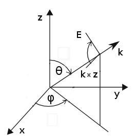
x axis	y	90	0	0
x axis	z	90	0	90
y axis	x	90	90	0
y axis	z	90	90	90
z axis	x	0	0	90
z axis	y	0	0	0

See Example 2 for details of use.

TSF_SKIP
boundary
Specifies boundary that should be excluded from TSF application. Parameter "boundary" is string denoting which boundary is being set (i0, j0, k0, in, jn, kn). Note that in principle TSF should be applied on all the boundaries to work properly, but in case of special materials or boundary conditions some boundary skipping can make sense.

SOURCE_LTSF
i_start j_start k_start i_end j_end k_end theta phi psi n_materials mat1_pos mat1_epsilon mat1_mu mat1_sigma mat_sigast .... mode (filename, values)
Plane wave source using layered total/scattered field formulation as published by I.R. Capoglu, G.S. Smith: IEEE Transactions on Antennas and Propagation 02/2008, 56:1. In contrast to SOURCE_TSF, here the material can be formed by N layers in z-direction (in present implementation only dielectric and non-absorbing). Incident wave however can cross the sample at angle as well. Layers need to be introduced both in parameters of the source and in material description files (as set MEDIUM_LINEAR or MEDIUM_VECTOR) and the values of material parameters need to match at LTSF boundary.
First six integers determine volume that is used for field propagation, theta and phi determine wave direction and psi its polarisation. This is followed by number of interfaces. For every interface its position in z direction and four material parameters are entered. By default the zero interface starts at z=0 and has permittivity of vacuum, so it does not need to be entered. Plane wave should start at vacuum. In order to create single free standing film we therefore need to enter two interfaces, upper and lower as seen in the example below. Next parameter, "mode", distincts again different source definition (same as for TSF). For "mode=0" a filename is provided pointing to a text file containing number of values N followed by N pairs of values step number - electric field value. N needs to be at least the total number of steps in simulation. For "mode=1" the source file is automatically generated (file "tmpsource" in the current directory) providing a sine wave source; the parameter after "mode" is therefore wavelength in meters followed by electric field amplitude. For "mode=2" the same happens for sine wave damped by a gaussian envelope, parameter "mode" is therefore followed by wavelength and by gaussian envelope width, given in integer steps of the simulation (e.g. 20), and then electric field amplitude.

As an example to create a plane wave (with a pulse time dependency and polarisation angle 0.3 rad) incident at angle on a free standing dielectric layer (in 200x200x200 voxels computational volume), use the following: SOURCE_LTSF 30 30 30 170 170 170 0.3 0.3 0.3 2 80 3 1 0 0 120 1 1 0 0 2 2e-7 50 5
Note that in this case the material parameters need to match the source, so e.g. using MEDIUM_VECTOR definition we can use this material file:
8 20 20 80 180 180 120 0 3 1 0 0

SOURCE_SF
theta phi psi mode (filename, values)
Plane wave source using pure scattered field formulation, working only for PEC interfaces. The parameters for source direction and data definition are the same as for TSF source. Note that SF source is not suported by GPU in present version.

See Example 3 for details of use.

SOURCE_TSFF
i_start j_start k_start i_end j_end k_end thetamax fdist polarisation n m mode (filename, values)
Z direction oriented focused wave source using total/scattered field formulation with multiple plane waves decomposition according to algorithm published in I.R.Capoglu, A. Taflowe, V. Backman, Optics Express 23 (2008) 19208. Six integers determine volume that is used for field propagation, thetamax determines maximal angle of incoming light, fdist the focal distance in voxel units. Polarisation angle of the incoming wave can be controlled by the following parameter. Integer parameters n and m determine number of plane waves to be integrated (more is better, values around 12, 36 should be already enough). Similarily to plane wave source, parameter "mode" distincts different source definition. For "mode=0" a filename is provided pointing to a text file containing number of values N followed by N pairs of values step number - electric field value. N needs to be at least the total number of steps in simulation. For "mode=1" the source file is automatically generated (file "tmpsource" in the current directory) providing a sine wave source; the parameter after "mode" is therefore wavelength in meters, followed by electric field amplitude. For "mode=2" the same happens for sine wave damped by a gaussian envelope, parameter "mode" is therefore followed by wavelength and by gaussian envelope width, given in integer steps of the simulation (e.g. 20), and finally electric field amplitude.

SOURCE_LTSFF
i_start j_start k_start i_end j_end k_end thetamax fdist polarisation n m n_materials mat1_pos mat1_epsilon mat1_mu mat1_sigma mat_sigast .... mode (filename, values)
Similar focused source to SOURCE_TSFF, however now dielectric material layers arranged in z direction can be crossed, similarly to SOURCE_LTSF. Note that in contrast to SOURCE_TSFF much more memory is needed for precomputation of the incident field and in present version you can easily run out of memory for larger systems or larger number of computation steps.

SOURCE_WAVELENGTH
min center max

Override automatic wavelength detection mechanism for sources. These (or automatically detected) values are used when listed material (e.g. silica) is used to pick the optical properties at right wavelength from the predefined values. Center value is used for materials that are predefined as lookup table, min and max values are used for materials where we have some dispersion model available.

Note that in present version every output needs GPU data to be synchronized with CPU, which can take significant time. For really fast simulations try to reduce frequency of data outputs.

OUT_FILE
filename.gwy
Set filename that will be used for outputing data. Gwyddion file (*.gwy) holds all data cross-sections (2d data).

OUT_POINT
Ex/Ey/Ez/Hx/Hy/Hz/All nskip i j k filename
Output values of given component of electric/magnetic field into text file (filename).

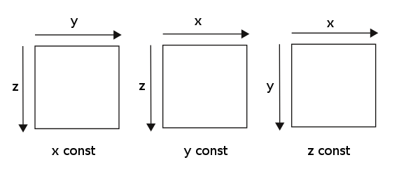
OUT_IMAGE
Ex/Ey/Ez/Hx/Hy/Hz/All nskip i j k description logscale/nologscale
Output image of plane cross-section. Which plane is used is determined by indices i j k; two of them must be -1. Logscale parameter is unused for now (but must be present). All results are saved to a .gwy file, skipping given number of steps (e.g. not outputing image in every step unless nskip=1). Description is a string shown for the channel in Gwyddion data browser.

Note that Gwyddion shows data with top-left corner being center of coordinates, orientation of axes on what is seen in Gwyddion is show below

OUT_SUM
component skip i_start j_start k_start i_end j_end k_end epsilon mu sigma sigma* filename
Output sum of electric field intensity (components: ex, ey, ez, all) or absorption (component: abs) extracted from bounding box and material with given properties (epsilon only used for this). If epsilon is -1, no control of this parameter is done and whole box is used. Parameter "skip" controls frequency of file output only (and sync with GPU eventually), values are calculated at each time step anyway and will be output for intermediate steps as well. At present this is tested only on CPU.

OUT_FORCE
skip i_start j_start k_start i_end j_end k_end filename
Output optical force acting on volume defined by six integers. X, y, and z component time dependence is output together with its values averaged over source period (source frequency is determined using FFT). Optical force is calculated using Maxwell stress tensor. No media should cross the boundary and scaterrer to be evaluated should be placed inside the evaluation volume.

NFFF
i0 j0 k0 i1 j1 k1 sum_from sum_to
Near-to far field calculation boundary definition. Needs to be within the computational volume. Parameters i0..k1 define the boundary position, sum_from and sum_to define the range of NFFF data summation when applied (not supported now). See example 3 for details of use.

NFFF_SKIP
boundary i_min/j_min j_min/k_min i_max/j_max j_max/k_max
Specifies area that should be excluded from NFFF calculation. Parameter "boundary" is string denoting which boundary is being set (i0, j0, k0, in, jn, kn), the next four numbers describe "upper left" corner and "bottom right" corner of the skipped area. Multiple calls of NFFF_SKIP can be used to exclude more areas on different boundaries, however at present only one area on each boundary can be set. Note that in principle NFFF should be applied on all the boundaries to work properly, but in case of special materials or boundary conditions some boundary or boundary area skipping can make sense.

NFFF_RAMAHI_POINT
i j k filename
Far field point designed for time values of electric field output. Can be outside of the computational volume even if it is entered in integer values representing position in computational volume (therefore values can be e.g. negative). See example 3 for details of use.

NFFF_SPHERICAL_AREA
theta_res phi_res radius theta_from phi_from theta_to phi_to savefile
Creates set of far field points designed for time values of electric field output. Set of (theta_res x phi_res) points are on a sphere of given radius (int integer i.e. voxel units), theta is declination and phi is azimuth. Parameter savefile determines whether to save all the farfield point dependencies or just put the total output into general output file (in Gwyddion format). As an example, considering a surface with normal oriented in z direction (negative), to cover whole half-sphere above sample for reflection scattering simulation by set of 20x20 points on sphere with radius of 1000 voxels, and not to save intermediate files, write

PERIODIC_NFFF
i0 j0 k0 i1 j1 k1 per_ifrom per_jfrom per_ito per_jto
Periodic near-to far field calculation boundary definition. Suitable namely for use with periodic boundary conditions of same dimensions. Uses only z planes (given by integer k0, k1) but repeats it as many times as given by integer span (per_ifrom, per_jfrom, per_ito, per_jto). Using periodic repeating values 0 0 1 1 gives the same result as conventional NFFF with skipped all the boundaries except single z plane. Values of periodic repeating can be negative, so e.g. values -1 -1 2 2 will produce result of 3x3 copies of calculated fields centered at the originally computed one.

PERIODIC_NFFF_SKIP
boundary i_min/j_min i_max/j_max
Specifies area that should be excluded from periodic NFFF calculation. Parameter "boundary" is string denoting which boundary is being set (k0 or kn as no other boundaries are used in periodic NFFF), the next four numbers describe "upper left" corner and "bottom right" corner of the skipped area. Note that in principle NFFF should be applied on all the boundaries to work properly, but in case of special materials or boundary conditions some boundary or boundary area skipping can make sense.

PERIODIC_NFFF_RAMAHI_POINT
i j k filename
Far field point designed for time values of electric field output in periodic NFFF. Can be outside of the computational volume even if it is entered in integer values representing position in computational volume (therefore values can be e.g. negative).

PERIODIC_NFFF_SPHERICAL_AREA
theta_res phi_res radius theta_from phi_from theta_to phi_to savefile
Creates set of far field points designed for time values of electric field output using periodic NFFF. Set of (theta_res x phi_res) points are on a sphere of given radius (int integer i.e. voxel units), theta is declination and phi is azimuth. Parameter savefile determines whether to save all the farfield point dependencies or just put the total output into general output file (in Gwyddion format). As an example, considering a surface with normal oriented in z direction (negative), to cover whole half-sphere above sample for reflection scattering simulation by set of 20x20 points on sphere with radius of 1000 voxels, and not to save intermediate files, write

PERIODIC_NFFF_SPHERICAL_AREA
20 20 1000 90 0 180 360 0

GPU
ngpus
Set number of graphics cards to be used (indexed as CUDA indexes them). If this command is not used or set to zero, calculation is performed on PC processor. See example 1 for details of use. Note that at present version use of multiple GPUs together is implemented, but untested.

UGPU
number
Set GPU with given index to be used for calculations (indexed as CUDA indexes them). This can be used for example to run several different calculations on different cards. See example 1 for details of use.

VERBOSE

0-4

Set text output (step by step), from full (4) to silent mode (0).

Examples

There are several examples distributed together with the source files, serving to test different software algorithms. Please note that if you have installed the Gsvit package into the standard location (e.g. /usr/share/gsvit/tests on Linux), the software runned as ordinary user won't have permissions to write the results. Therefore, we recommend to copy the respective test directory to the home directory owned by the user and run the computation from this location.

Basic program operation
Total/scattered field source, PEC sphere
Scattered field source, PEC sphere
Near-to-far field transformation
CPML boundary condition
Periodic boundary conditions