Tutorial:
FDTD & GPU
Yee's algorithm
Sources
Materials
Boundary conditions
Near-to far field
Application notes
Application note: Transmission diffraction grating
As an example of extensive use of Near-to-Far Field (NFFF) transformation we dicuss modeling of a diffractive optical element performance. Scattering from diffraction gratings and similar periodic structures can be evaluated analytically to some extent (e.g. for ideal gratings). However, for analysis of different defects, like shape of a single groove, roughness or faults in periodicity, we need to use some numerical technique. FDTD is one of the options, however as the grating is periodic it is very suitable also for RCWA (the best option) or FEM.
Transmission through single aperture
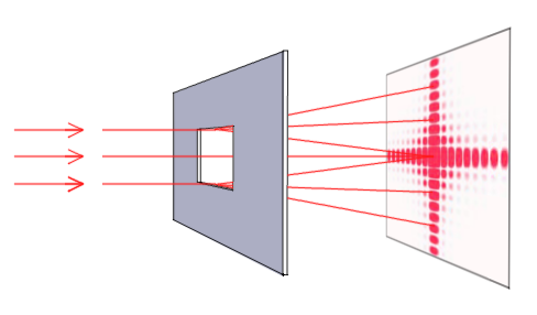 |
First, consider a single hole in an opaque screen - rectangular aperture. If a light is illuminating the screen on the other side a diffraction pattern is formed behind it (and can be seen on the screen located behind). With smaller ratio between aperture size and wavelength this effect becomes more pronouced and angular spacing between diffraction maxima is larger. As the diffraction pattern can be calculated analytically (at least in Fraunhofer diffraction approximation), we can use this model for comparison of FDTD result to analytical results. |
If we consider x and y as axes on the screen where diffraction pattern is seen, the intensity space distribution varies as

where p and q are aperture dimensions, r is distance from aperture to screen center, A is related to incident field amplitude and k=2π/λ where λ is the incident light wavelength.
|
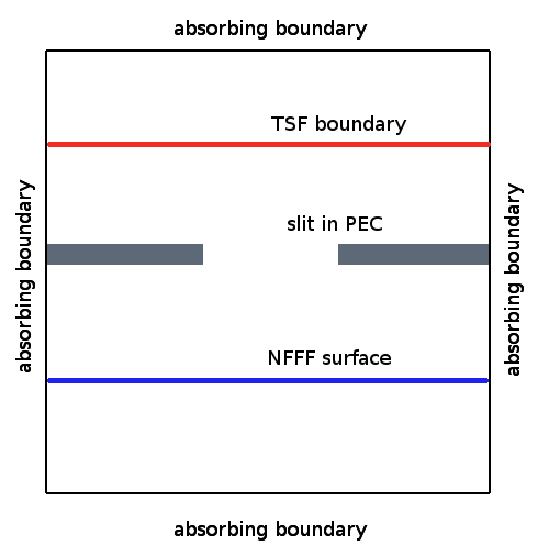
Image on the right shows scheme of the computational volume used for the simulation (a cross-section). We use a parallelepiped bounded by simple absorbing boundary conditions. A plane wave source is established using Total/Scattered field approach (TSF), but only single plane is used to excite the plane wave (all the other faces are skipped). Grating material is introduced as vector material - by using one perfect electric conductor (PEC) parallelepiped to create thin non-transparent plate and one smaller vaccum parallelepiped to create a rectangular hole in it. Near-to-far field transformation (NFFF) integrated from plane behind the aperture is used to calculate far field radiation pattern. Preserving both TSF source and NFFF integration plane close to metal plane helps to minimize influence of finite plane wave and metal plane size. |
 |
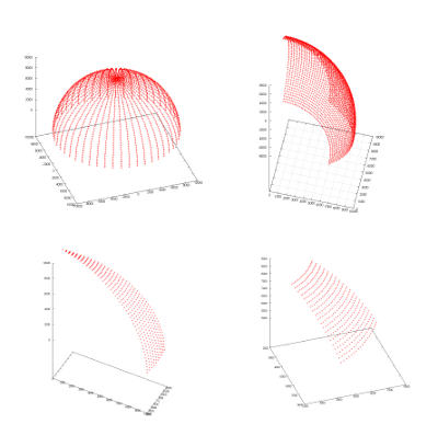 |
Far field radiation pattern is evaluated on a sphere (or its part) with prescribed radius, here approximately 3 cm. Spherical coordinates are used for this, so the output of calculation spans some values of θ (in range of 0-360) and φ (in range of 0-180), so the results can contain different parts of a sphere as shown for different settings on the left image. As a result we get a 2D diagram of scattered light intensity that can be visualised or processed in Gwyddion. There are two possible ways how to create source. We can use a monochromatic plane wave (e.g. 633 nm) and evaluate the scattered light at this wavelength directly. Alternatively, we can use a broadband pulse, here a gaussian function, determine its spectral dependency by Fast Fourier Transform (FFT) and determine spectral dependency of the computation output (again by FFT). This gives us the spectral dependency of scattered light from a single computation. |
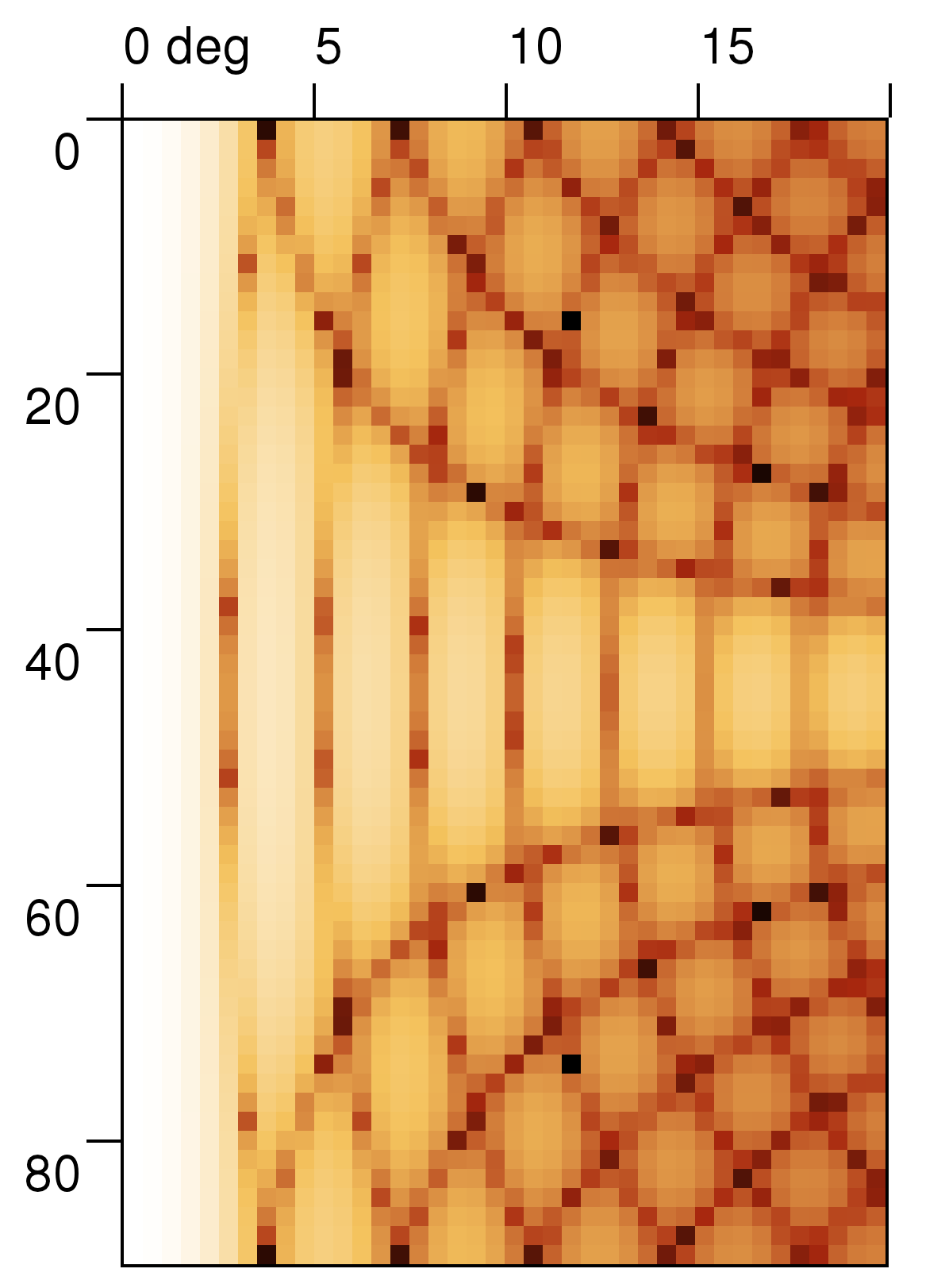
As a result we obtain a far field radiation pattern as shown below on the right image (analytical result is in the left image). Both images are in logarithmic scale for intensity false color plot. Only a single lobe is calculated (i.e. a quarter of the whole pattern that is four times repeated in 0-360 degrees due to the fact that aperture is square). We can clearly see the diffraction pattern and we can compare it with analytical result.
 |  |
 |  |
Transmission through a grating
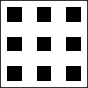 |
Grating is formed by equally spaced set of apertures. An image of ideal diffraction grating aperture locations is shown in the left figure (ideally the number of apertures in every direction would be infinite). Grating is again made from non-transparent material and as light goes through its slits (shown by black color) it is diffracted. Due to constructive and destructive interference the transmitted light has strong dependency of intensity on propagation angle, so if we place a screen behind the grating we will see equally spaced set of points - diffraction maxima - modulated by diffraction of single aperture forming the grating. To model diffraction grating we use the same approach as in above example, however periodic boundary conditions are now used in xy direction. To evaluate far field scattering pattern, a periodic NFFF computational boundary is used, which means that local fields on integration boundary are copied as many times as requested, simulating much larger periodic structure. |
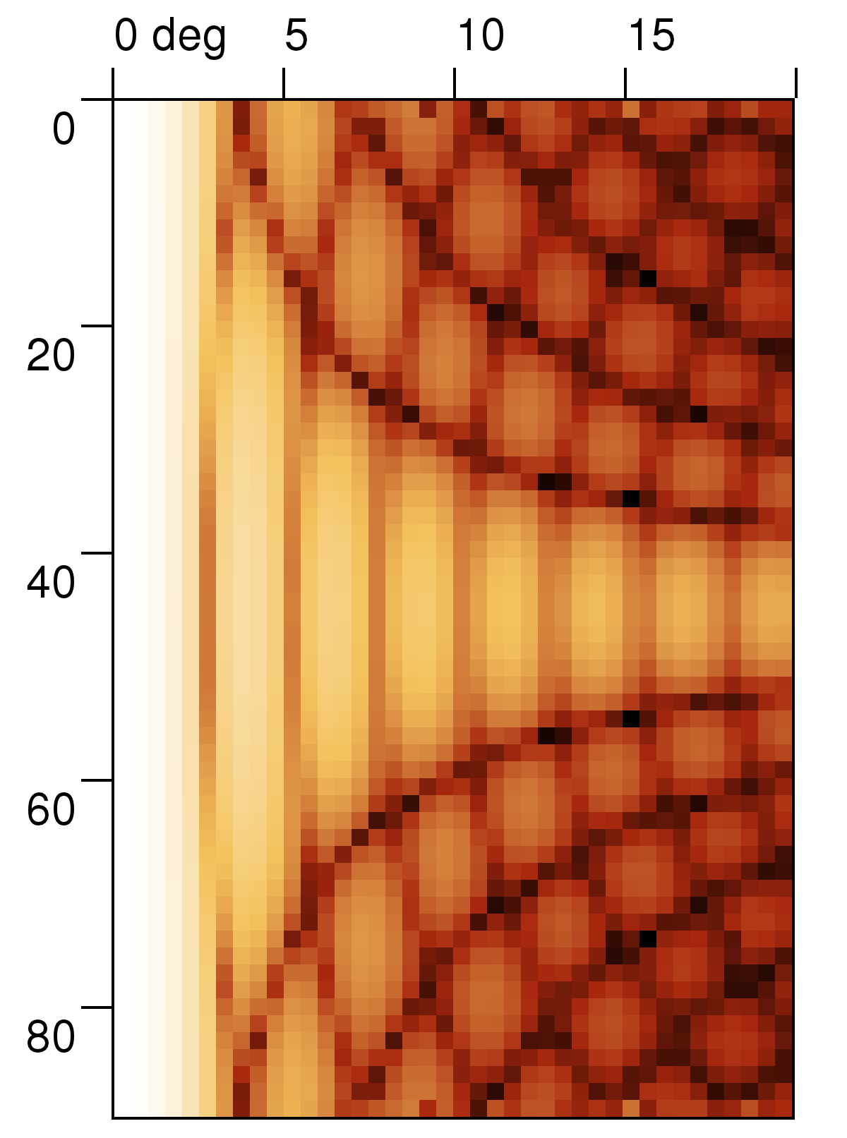
The whole pattern as simulated for grating spacing to wavelength ratio of approx 10:1 and finite size of 13x13 holes is shown below, both in normal and logarithmic scale (note that in contrast to aperture simulation results now the θ axis is the horizontal one).
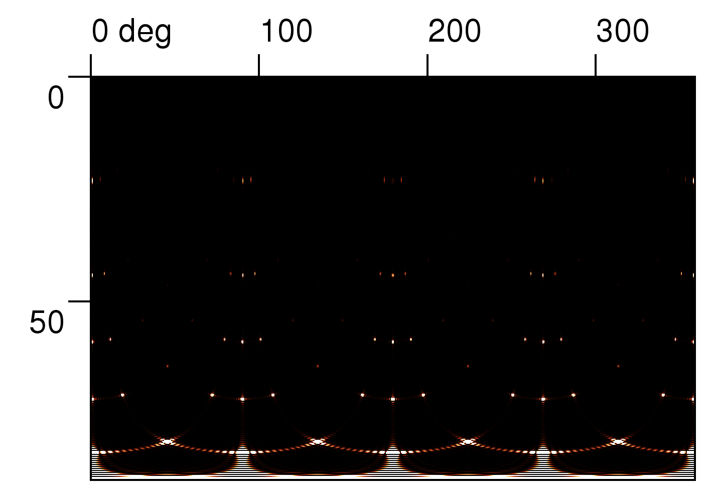 |
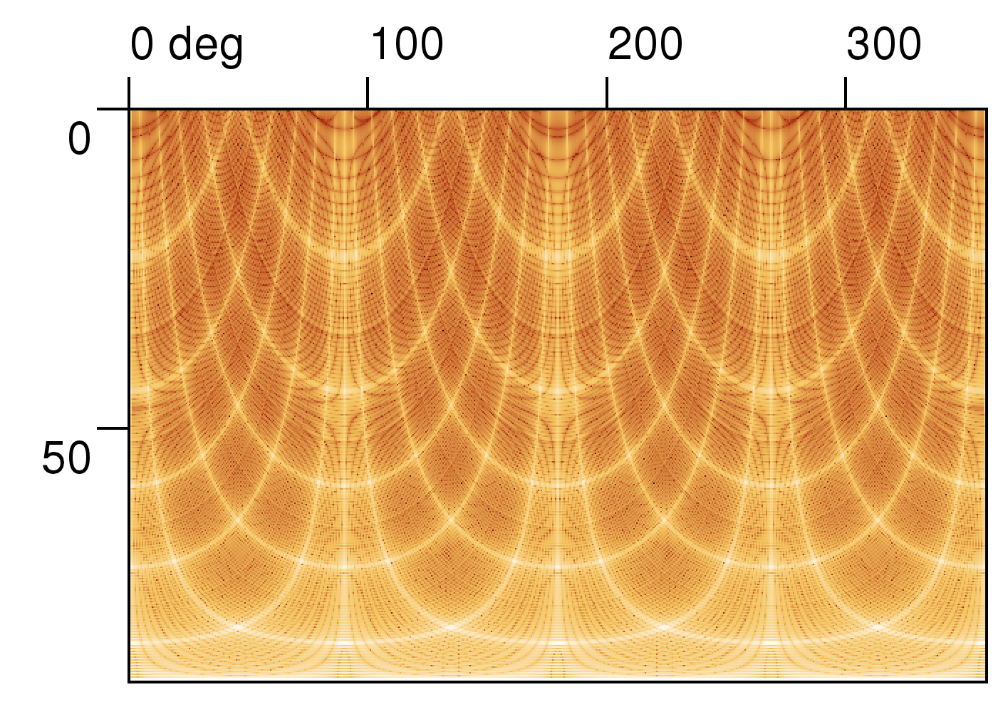 |
Analytically this can be written for diffraction angles θ1 (in the x direction) and θ2 (in the y direction) as

where a1 and a2 are grating hole spacing in x,y direction and N1 and N2 are number of holes in these directions; the rest of symbols is same as in aperture equation.
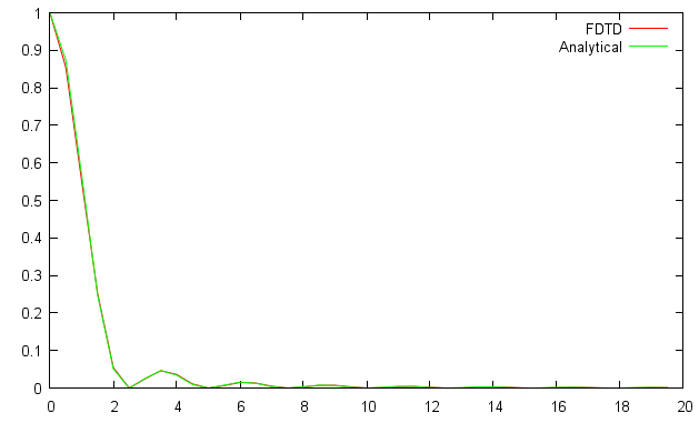
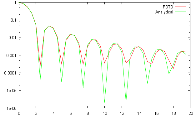
Even if it would be in principle possible to calculate the same images also using FDTD, the number of far field points with the same resolution would be around million which is already significantly slow in present version of GSvit. Therefore we had compared result only on a single profile in x direction again, similarily to how the aperture intensity graphs were obtained. Results are show below (x axis is in degrees)
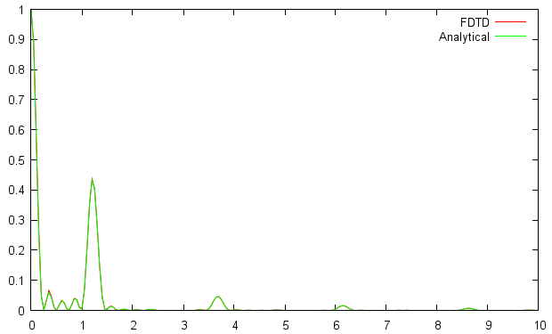 | 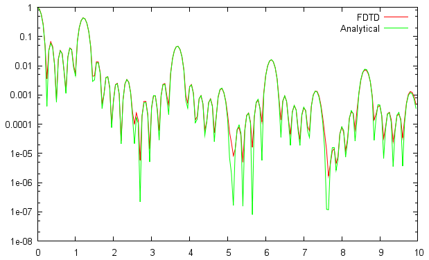 |
To setup calculation similar to those shown in this example you can try this XSvit example and related files
.(c) Petr Klapetek, 2013
