
|
Main page Tutorial: FDTD & GPU Yee's algorithm Sources Materials Boundary conditions Near-to far field Application notes | Chapter 3: SourcesTo perform a computation we need to setup at least single source of electromagnetic field. The simplest source is a point one, which is physically similar to a small dipole. More rigorous is an electric or magnetic current source which has exactly the same funcionality as the electric or magnetic dipole. If we need a plane wave to interact with our computation volume, we are no more able to use a set of point sources (unless we have extremely large computational volume which is unrealistic. Special techniques need to be used, for example one known as total/scattered field or scattered field. Both approaches are based on addition and eventually subtraction of precomputed plane wave to/from some points in the computational volume. In total/scattered field (TSF) technique we draw a boundary around the area where we need the plane wave and we add the plane wave on one side and subtract it on other side (depending on wave traveling direction). There can be anything inside TSF volume as there are no special algorithms run there. In scattered field (SF) formulation, we only add the plane wave on tangential electric field components of interface between conductor and non-conductor, simulating the fact that in real world there are currents cancelling the tangetial components of electromagnetic wave generated on such interface. At it's simplest variant this technique is therefore not suitable for dielectrics and it is used for calculations consisting of perfect electric conductors in a free space. However, comparing to TSF, it can provide more accurate results for scattering calculations in these cases. In Gsvit, there are point, TSF and SF sources implemented at present. SF source is working only with PEC (defined as tabulated material). See the parameter documentation for details, some of the preinstalled examples or click on one of the images below to see how use these sources. 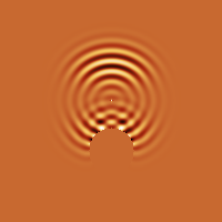

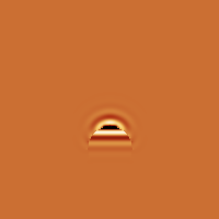
Point source (left), total/scattered field source (center) and scattered field source (right) hitting a perfect electric conductor sphere. Note that in TSF and SF source the plane wave pulse is traveling from top to bottom in the shown cross-section of computational volume and boundary of TSF volume can be clearly seen. Click on image to see the parameter file and other linked files for running the same example in GSvit (c) Petr Klapetek, 2013 |