Local field enhancement close to a metallic rod

Summary

We will setup computational volume with a metallic rod in the center, illuminate it by a plane wave and we will observe local field enhancement at the side of metallic rod. Realistic metal model will be used for the rod treatment, representing silver. This is a model similar to what is used in application example for plasmonic nano-antennas.

What can be tested:

• Real metals performance
• TSF source
• Summing output from certain volume

Setup all this with XSvit

Note that some of the screenshots might be from an older version of XSvit.

Start the XSvit application and setup the computational volume in this way:

• Computational volume size 240x240x100 voxels, discretisation 1.7, 1.7, 1.7 nanometers.
• 8000 computation steps
• Liao boundary conditions everywhere.
• TSF source spanning from 10 to 230/90 in xy/z Orientation angles (theta, phi) set to zero, polarisation (psi) to 90, wavelength chosen between 600 and 1300 nm.
• Summing output from box spanning from (40, 110, 40) to (50, 130, 60), component "All" (this means total field magnitude), so we want to know the field at the neighbourhood of the metallic rod.
• Some image outputs at center of the computational volume to see the calculation progress.
• Vector material file with a single object:
  
  8 60 110 35 180 130 65 4 1.1431 1.3202e16 1.0805e14 0.26698 -1.2371 3.8711e15 4.4642e14 3.0834 -1.0968 4.1684e15 2.3555e15
  
  which means a single silver parallelpiped approximately in the center of computational volume, using CP model for metal dispersion properties.

We refer to basic appplication use example for details how to adjust all these settings.

After setting all this the complete setup should look like this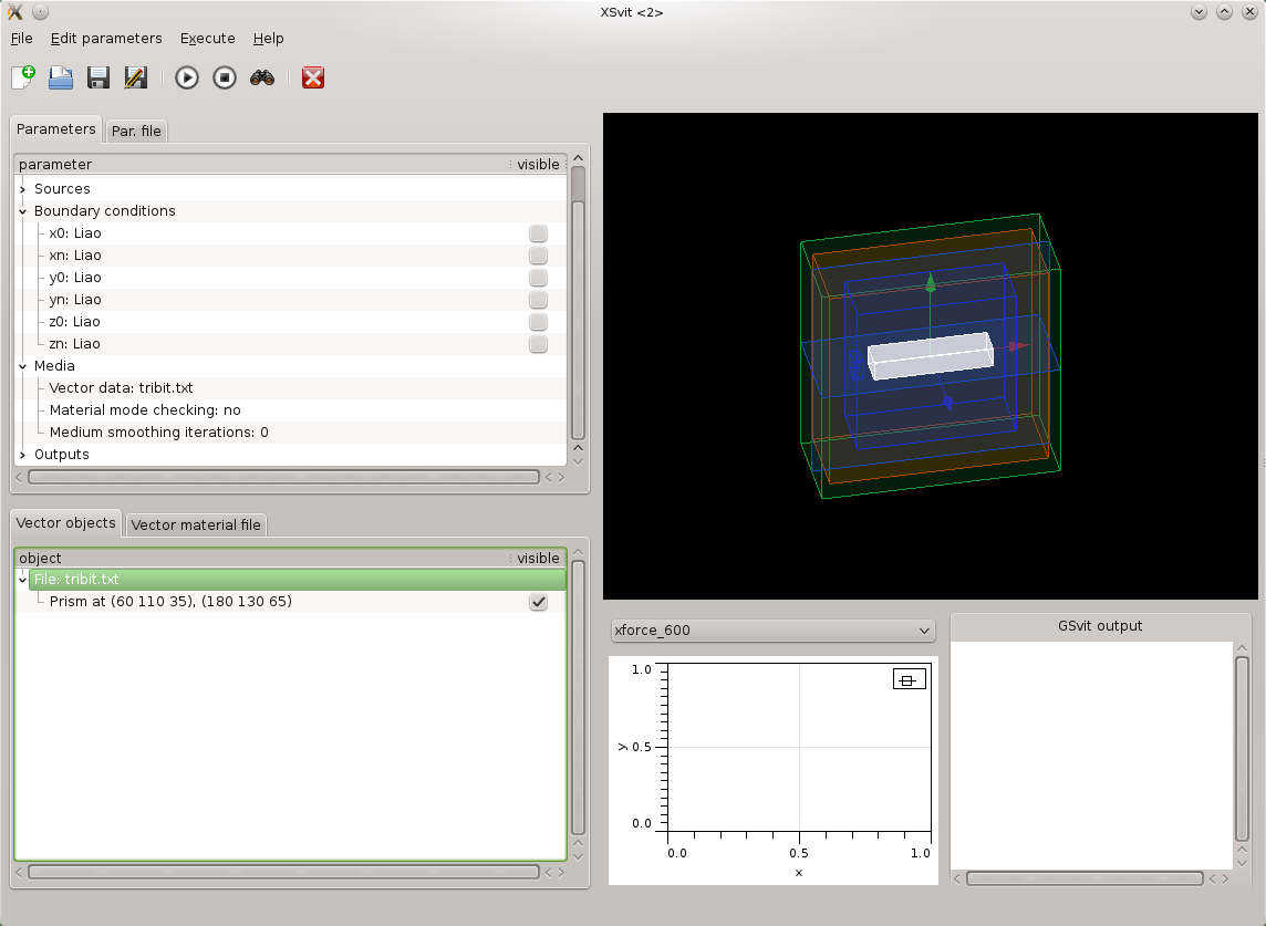

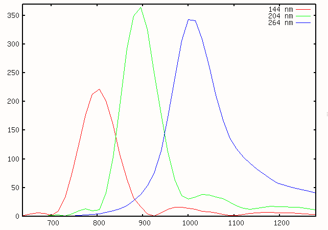
Then we can save all files and run the computation. As a result we get time dependence on the summed electric field; we can see that during the computation this value converges to some oscillatory behavior. When we run similar computation for different wavelengths and then plot the average of converged sum values over a period together into a spectral plot, we can see the spectral dependence of the field enhancement in nanorod neighbourhood (three such spectra are shown here for different rod lengths).

Here you can download sample parameter file and vector material file for this example.

Back to the documentation.