
|
News Features Documentation Download Participate |
GSvit v 1.7 graphical user interfaceGSvit architecture is based on use of computational core (GSvit) and a GUI (XSvit). This page provides documentation for the graphical user interface, you can also check the documentation for computational core. InstallationPlease see the download page. Running the graphical user interfaceGraphical user interface does not require any command line arguments (starting with a new parameter file) or alternatively you can pass a parameter file as an argument (then it will open it). All the rest is done via different controls and dialogues within the software. Quick startCheck the basic program operation example to run your first computation. Other examples are linked at bottom of this page. DocumentationXSvit is primarily a viewer of parameter files suitable for GSvit FDTD calculations. It cannot do anything except it, however it can simplify the process of parameter file creation and modification as it serves as a viewer and basic editor of parameter files. Its GUI is shown in the following image: 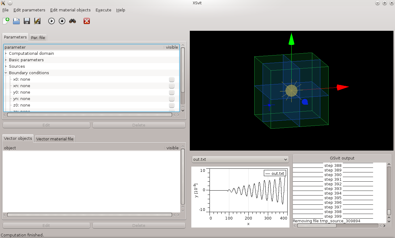
Technically the primary data in XSvit are the parameter file that is shown in the "Par. file" tab in left side of the screen. This represents the data directly as are used in GSvit. While loading this file or reloading it after any modification, XSvit goes through the parameters in it and constructs list of entries shown in tab "Parameters". By clicking on any of these entries, or by using the Edit parameters menu, we can adjust parameters or add some more of them. If we do so, parameter file is automatically written into a temporary location and reloaded back. This is to guarantee consistency of the parameter file with GSvit. As an alternative, we can also edit content of "Par. file" tab multiline text entry. If we do so, parameter file is dynamically reloaded as we type (and all the entries in "Parameter" tab are again refreshed). Note that the parameter file used within all the modifications is temporary, so it must be saved prior to computation or exiting the software. Similarily to parameter file, there is also material file and list of material entries representing "vector material" if such is used in the computation. Again, material file is the primary source of information, however you can edit material objects by Edit materials menu. All this is related to so called vector material file (see GSvit documentation), which is only one of ways of including a material in computational domain Which material file to show in materials list is governed by parameter file entry called "vector material". Therefore, chaning this entry also leads to loading another material file. Current temporary material file is saved automatically when we save the parameter file to assigned "vector material" file. Main screenThere are few key elements of the main screen that appear when you start XSvit:
Note that at this version of XSvit, some amount of warnings and errors is still output to console, namely those related to parsing the parameter file (that is done by GSvit functions where a console output is normally used). This will change in future versions to get rid of the console (which is too unusual on Windows). Parameter file related dialoguesThere are many simple dialogues that can be used for entering different computation parameters. They can be invoked by double clicking on an entry in list of parameters at left side of the screen, by Edit button, or, for newly set objects/settings by Edit parameters menu. Most of the dialogues are shown in some of the examples (see bottom of this page) in practice, here is their list as well. Note that many more details about realisation of different parameters are in computational core documentation. Parameter settings Global parameters that can be set are location of GSvit and Gwyddion executable. These are used for calling GSvit and Gwyddion directly from GUI, if we only want to create parameter files and run the computation and output visualisation elsewhere, we don't need them. Please note that on Windows OS the default installation path for GSvit binary is typically C:\Program Files (x86)\GSvit\bin\gsvit.exe. 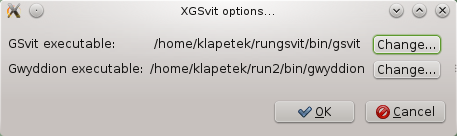
Computational domain settings There are two main computational domain parameters: voxel size (also called resolution in the documentation) and voxel spacing. Voxel size can be any (for any direction), however note that GSvit is 3D FDTD solver, so settings any dimension to e.g. 1 does not convert it to 2D solver. Voxel spacing should be the same for all the dimensions in this version, using different spacings is untested, even if in principle FDTD allows it. If we are in vacuum, voxel spacing should be at maximum 1/10 of the wavelength used. 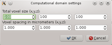
Basic parameters settings Several basic parameters influence the whole computation (all the algorithms): number of Yee algorithm steps (real time step is calculated automatically), verbosity level (0...3), use of multithreading based on OpenMP (-1...N) where -1 means use of all the available cores, and use of any of the available graphics card instead of processor. Note that verbose level should not be 0 to see anything in the text output (e.g. in log window in the GUI). On the other hand, high verbosity level might lead to some delays in GUI visualisation on MS Windows, so value of 1 seems to be optimum. If you have doubts whether graphics card is usable, you can run gsvit test 0 to perform basic test of Nvidia CUDA capable devices. Cards are counted from zero. 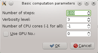
Boundary conditions Computational volume typically needs to be terminated somehow and the following dialogue is used to set the boundary conditions. Different options can be chosen, starting from nothing (which reflects waves) up to Convolutional Perfectly Matched Layer conditions (for details see CPML boundary condition example). Note that even if in principle any boundary can have different boundary condition applied, it is not guaranteed that all the combinations (e.g. Liao + CPML) are working together properly. This dialog can be used also to set some boundary conditions within the material, now only peridic boundary conditions. To do so, you must specify where from and where to the space should be treated as periodic. 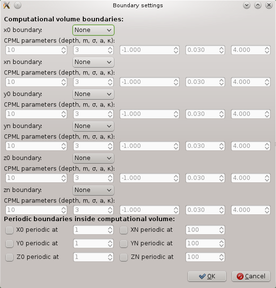
Input of geometry of media There are two ways how to input objects in this version of GSvit. These can be defined voxel-by-voxel for all the voxels in the computational domain or defined using discrete objects, here also called as vector data (spheres, cubes,... up to tetrahedral meshes). Voxel-by-voxel data are not further visualised in XSvit, vector data are loaded automatically on basis of settings in this dialogue to the bottom widget showing material entities. 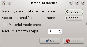
Output settings Main general output setting is the output file where all the cross-sections (images) go to. It is Gwyddion file so it can be opened only by Gwyddion. 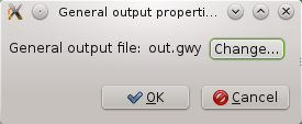
Point source A simple dipole-like point source realised by setting field quantities in a single cell to a prescribed time dependency. We need to set its voxel position and waveform, that can be both loaded from a text file (containing total number of steps followed by sequence of these entries: index Ex Ey Ez Hx Hy Hz). This file ca be also automatically generated providing a sine wave source or sine wave damped by gaussian envelope. Finally, two parameters theta and phi determine the source orientation. 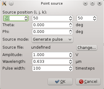
Scattered field source Scattered field source creates a plane wave by introducing its oposite to every face of a perfectly electric conductor. To use it you first need to have the conductor somewhere in your computational domain, and then also set the orientation of wave by the following dialogue. Other source conditions are same as for point source. For orientation details see the computational core documentation 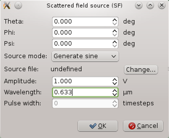
Total/scattered field source Plane wave can be also injected on some virtual boundary inside computational domain and removed at the other side. This approach is calle Total/scattered field source. To setup it we use the same parameters as to scattered field source, adding only definition of the virtual boundary where it is added/subtracted. 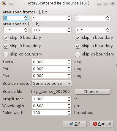
Focused total/scattered field source This represents z direction oriented focused wave source using total/scattered field formulation with multiple plane waves decomposition according to algorithm published in I.R.Capoglu, A. Taflowe, V. Backman, Optics Express 23 (2008) 19208. In addition to definition of virtual boundary where it is added/subtracted, we need to define maximal angle of incoming light, focal distance in voxel units and wave polarisation angle. Integer parameters n and m determine number of plane waves to be integrated (more is better, values around 12, 36 should be already enough).
Layered total/scattered field source Plane wave source using layered total/scattered field formulation as published by I.R. Capoglu, G.S. Smith: IEEE Transactions on Antennas and Propagation 02/2008, 56:1. In contrast to TSF source, here the material can be formed by N layers in z-direction (in present implementation only dielectric and non-absorbing). Incident wave can cross the sample at angle as well. Layers need to be introduced both in parameters of the source and in material description files and the values of material parameters need to match at LTSF boundary. In present GUI only two interfaces can be set (GSvit itself could handle any number of layers). Note that the source starts always in vacuum, so to add single material layer we need exactly two interfaces (one for upper boundary and one for lower boundary). 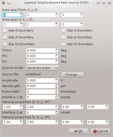
Layered and focused total/scattered field source A mixture of TSFF and LTSF source, i.e. focused source that can travel accross layered media. GUI is a combination of settings from both the sources (see above). 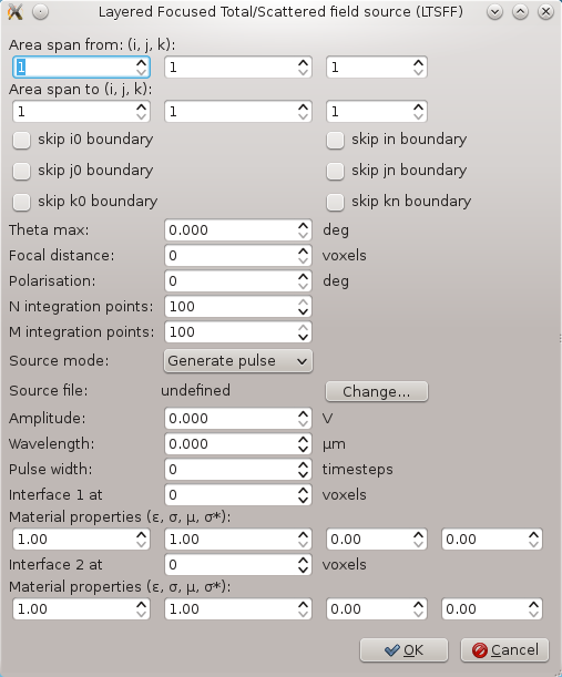
Point output A simple point output providing text file with specified data extracted from specified position. It does not need to be generated at every step (in some steps it can be skipped), which is useful namely when working with GPU (all the outputs lead to possibly unnecessary communication between graphics card and RAM). 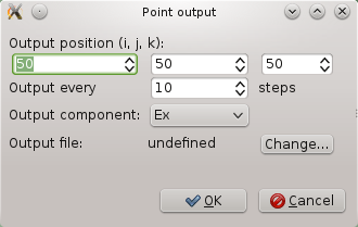
Image output Image output going to general output file. It always makes a cross-section, so its orientation and direction can be specified. Description is a string shown for the channel in Gwyddion data browser. 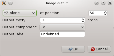
Plane output Same output as for image, but now going to a separate binary or ASCII file. It always makes a cross-section, so its orientation and direction can be specified. At every step (or coarser, depending on skipping settings) it makes a new file using the basename and step index. Start and stop settings can limit the output extent. 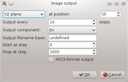
Summing output Output sum of electric field intensity (components: ex, ey, ez, all) or absorption (component: abs) extracted from bounding box and material with given properties (epsilon only used for this). If epsilon is -1, no control of this parameter is done and whole box is used. Skipping controls frequency of file output only (and sync with GPU eventually), values are calculated at each time step anyway and will be output for intermediate steps as well. At present this is tested only on CPU. 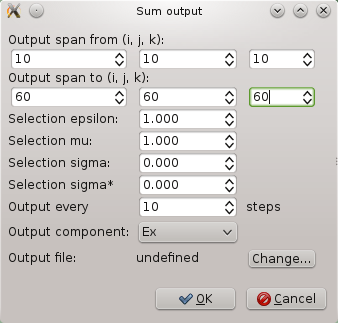
Volume output Output volume information about field components, material components (components: ex, ey, ez, hx, hy, hz, all, material) or absorption (component: abs). Skipping controls frequency of file output only (and sync with GPU eventually), ouput is performed only between start and stop step (-1 in these parameters means starting in first step and stopping in last one). Volume information can be binary or ASCII. Binary file is formed by 3D array of doubles that can be visualised e.g. by Paraview. ASCII output starts with header informing about voxel dimensions and selected component. 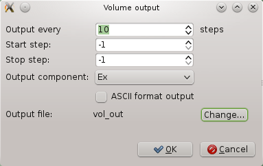
Force output Outputs optical force acting on volume defined by six integers. X, y, and z component time dependence is output together with its values averaged over source period (source frequency is determined using FFT). Optical force is calculated using Maxwell stress tensor. No media should cross the boundary and scaterrer to be evaluated should be placed inside the evaluation volume. 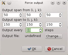
Near-to-far field transform basic settings Defines integration boundary for calculating far field values using time domain Near field to far field transform (NFFF). Sometimes it is useful to skip some part of boundary (or whole boundary) even if it is non-physical. In this case you can enter the area which should be skipped from the boundary (for every boundary independently). 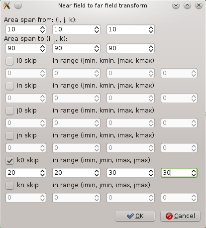
Near-to-far field output point Sets the position of far field integration point using NFFF. 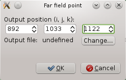
Near-to-far field output area Sets the generated set of far field points. Points are part of a sphere with defined voxel radius, with span given by theta and phi angles. 
Periodic near-to-far field transform basic settings Periodic NFFF is designed to be used with periodic boundary conditions and integrates the NFFF values from predefined number of repetitions of calculated far field values. It can be therefore used e.g. to calculated field from a grating while field over single pit is only calculated by Yee's algorithm. 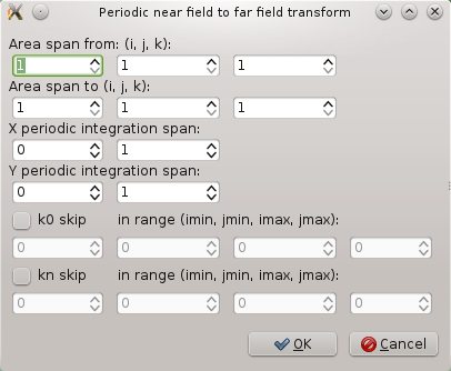
Periodic near-to-far field output point Sets the position of far field integration point using PNFFF. 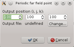
Periodic near-to-far field output area Sets the generated set of periodic far field points. Points are part of a sphere with defined voxel radius, with span given by theta and phi angles. 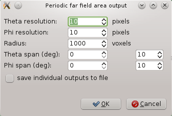
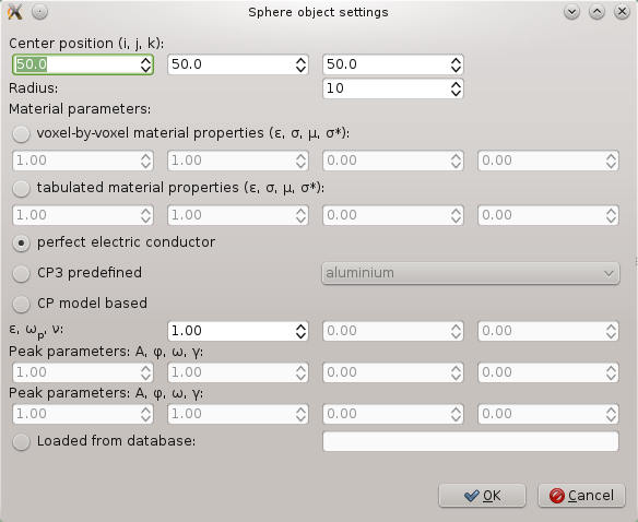
Material objects related dialoguesTo add an object to computational volume you can use Edit material objects menu, to edit it, double click on entry or click to "Edit" button while the entry is selected. To delete an entry, select it and click on "Delete". Note that there is no undo implemented up to now. Alternatively, you can write the vector material file directly (or, of course to do it in external editor or to prepare voxel-by-voxel file). Practically this means writing entities like 4 20 20 20 50 10which means adding a perfect electric conductor sphere of radius 50 voxels to position 20,20,20. For details see computational core documentation or some of the examples. Material object dialogues are numerous and in fact very similar. As an example, a sphere dialogue is shown below. First, object geometrical parameters in voxel coordinates are entered (here position and radius), then, material properties are assigned to this object. Details on different material properties regimes can be found in GSvit documentation, briefly said there are following options:
ExamplesBasic program operation There are also several basic examples distributed together with the application. to test different software algorithms. Please note that if you have installed the Gsvit package into the standard location (e.g. /usr/share/gsvit/tests on Linux), the software runned as ordinary user won't have permissions to write the results. Therefore, we recommend to copy the respective test directory to the home directory owned by the user and run the computation from this location. (c) Petr Klapetek, 2013 |