Near field to far field transform example

Summary

We will use cubic volume with Liao absorbing boundary condition and point wave source. Outputs will be cross-sections to a Gwyddion file and a point output. At the same point the field value will be calculated using Near Field to Far Field transformation.

What can be tested:

• NFFF operation, try different NFFF integration boundary sizes and shapes

Setup all this with XSvit

Note that some of the screenshots might be from an older version of XSvit.

Start the XSvit application and setup the computational volume in this way:

• Computational volume size 100x100x100 voxels, discretisation 1e-8, 1e-8, 1e-8.
• 900 computation steps
• Point source in computational volume center with orientation angles (theta and phi) set to zero, generated gaussian pulse wave with amplitude 1V, wavelength 488 nm and length 100 steps.
• Eventually some image output just to see that something is happening, but not necessary for this example.
• Point output (component = All) at position 60,70,80.

We refer to basic appplication use example for details how to adjust all these settings

At this moment we can add the NFFF integration area and NFFF output point. Near-Field to Far field transorm is typically used to calculated the field values outside of the computational volume, so we can extend our results to distance that could be never calculated by FDTD. However it is valid also inside the computational volume, so we can directly compare FDTD output to values calculated by basic Yee algorithm. Therefore we will start with adding NFFF output point at position 60,70,80 (same position where we have the regular point output) using menu item Edit parameters->Add NFFF point: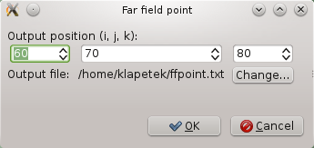

After adding the far field point new block of entries appears in the list of parameters and also the far field point can be shown in 3D view by a line pointing from center of computational volume to that point. We still need to adjust parameters of the NFFF integration domain, namely its integration boundary, that should enclose all the sources and scatterers, but not enclose the output points. Here we have chosen volume defined by top/left/front corner 30,30,30 and bottom/right/back corner 70,70,70. This parameter is set by clicking on "NFFF box" entry above the newly added far field point entry: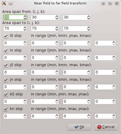

After all this we can see all the output points, source and NFFF box in the 3D view: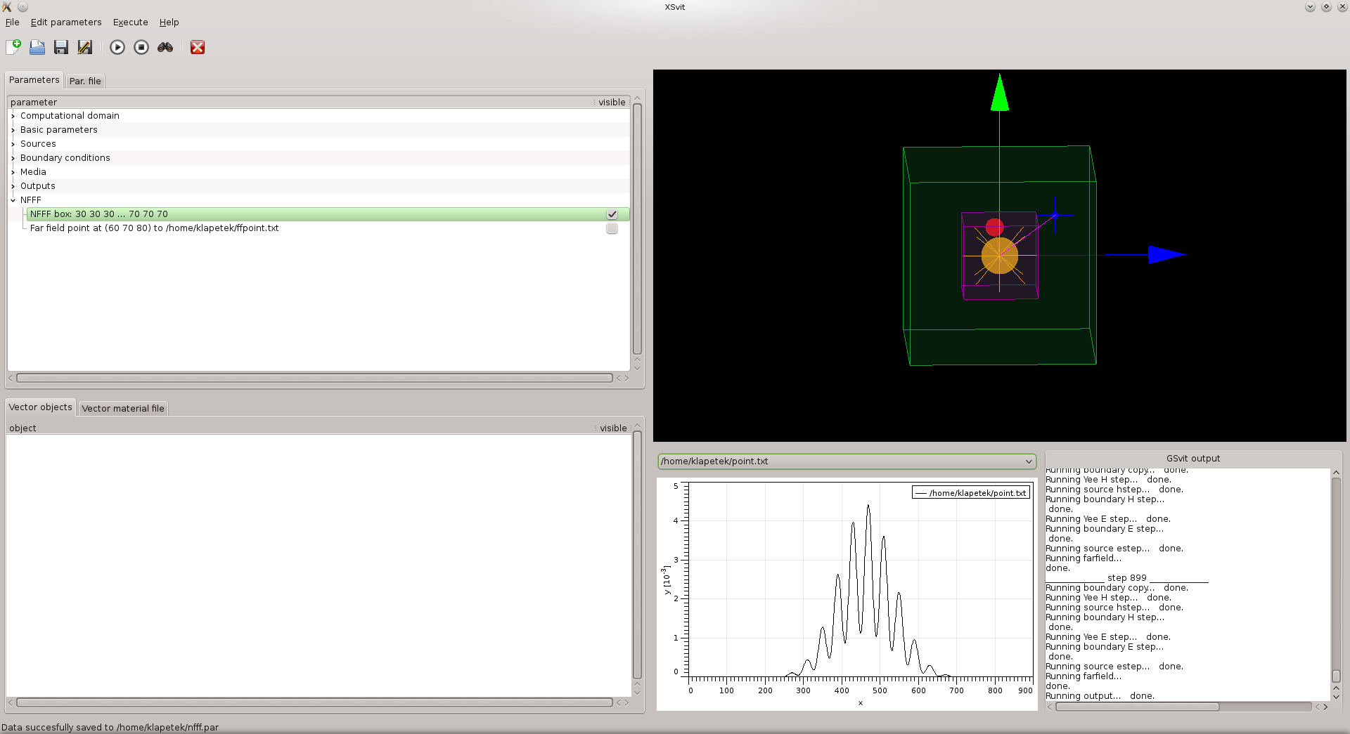

Then we can save the file and run the computation. We can see the point output values directly on the graph, however to compare the direct and the far field output it is easier to use an external application, here Gnuplot: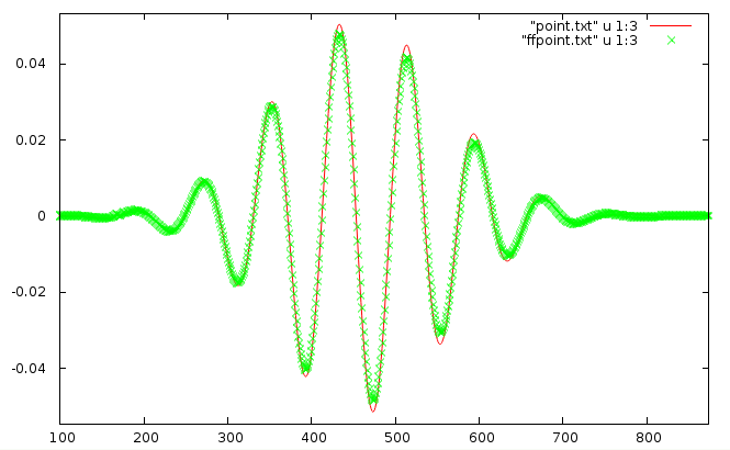

We can play with integration boundary settings to get the best match, generally it should be enclosing the sources and scatterers tight to get better results, however there are certainly some limits when too small integration boundary will lead to some numerical errors (as the number of integration points will be too small).

Download parameter file for this example: xex18_4.par

Next example

Back to the documentation.