
|
News Features Documentation Download Participate |
Convolutional perfectly matched layer boundary conditionSummaryWe will setup cubic volume with Convolutional Perfectly Matched Layer (CPML) boundary condition and a point source. What can be tested:
Setup all this with XSvitNote that some of the screenshots might be from an older version of XSvit. Start the XSvit application and setup the computational volume in this way:
We refer to basic appplication use example for details how to adjust all these settings In order to use CPML boundary we click on any of the boundary conditions entries in parameters list. Preset values of CMPL parameters should be fine for this application. Note that setting sigma to -1 leads to automatic estimation of the best value, based discretisation and timestep. 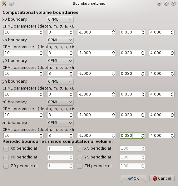
After setting all this we can see the estimated sigma values already in the list of parameter entries. 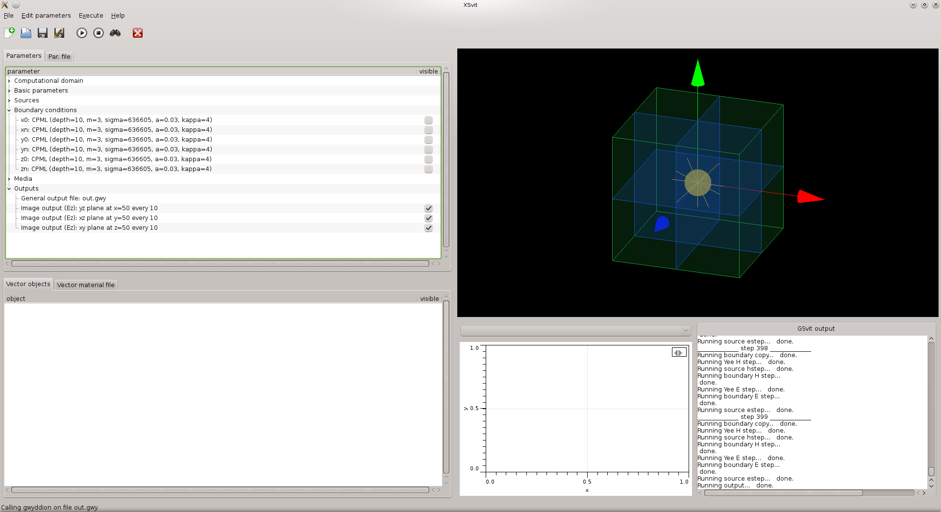
Then we can save the file and run the computation. In the output we can see that the wave is damped at the boundaries to zero. Note that CPML is not working only at boundary, but up to some depth (here 10 voxels). This should be considered while adding some objects or sources close to the computational space boundary. 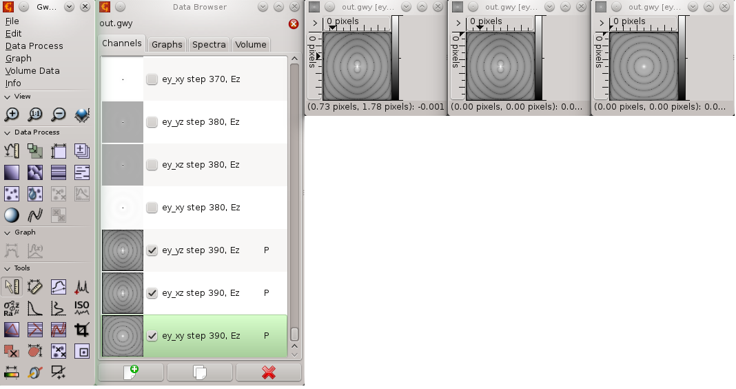
CPML is generally much better absorbing boundary condition than simple second order one (Liao), however it is also much more computationally demanding. Efficiency of its use therefore depends on application. CPML can work with dielectric media in it, so we can also simulate e.g. halfspace with some permittivity and wave will be damped even there. To test this, click on "vector material file" tab at the bottom, and add this line 8 0 0 65 100 100 100 0 3 1 0 0This means adding a rectangular area spanning from 0, 0, 65 to 100, 100, 100, and having relative permittivity of 3, relative permeability 1 and zero losses. Then we save this material file using menu entry File->Save material file as... (here we called it halfspace.txt) and we click on some of the media entries in the parameter list to add this file as vector medium. After running the computation we can get this output: 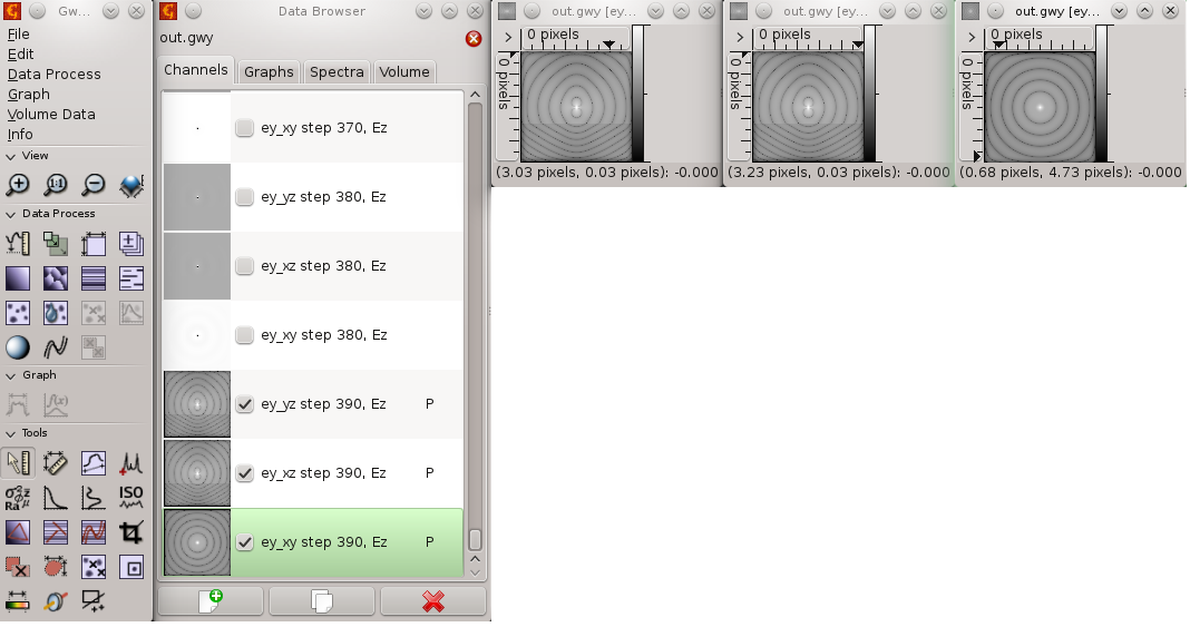
We can see that the wave is damped in both the halfspaces. Download parameter file for this example: xex18_5.par (c) Petr Klapetek, 2013 |