Main page
Tutorial:
FDTD & GPU
Yee's algorithm
Sources
Materials
Boundary conditions
Near-to far field
Application notes
| Application note: Rough surface scattering
In this example we will use GSvit to simulate scattering from a highly absorbing sample
(e.g. metallic).
Calculation procedure is very similar to reflection grating example, we again use
a height field to setup measurement volume material parameters, however here we do not apply
periodic boundary conditions as the surface is not periodic (and we do not want to introduce artificial
periodicity to the results).
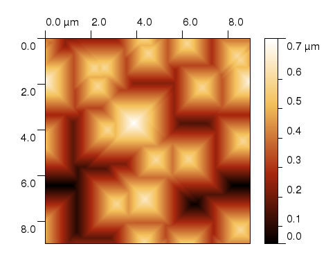 |
In the left figure a topography of randomly rough surface similar to one used in solar cell manufacturing is displayed.
Surface is formed by randomly placed facets of size similar to visible wavelength, so we cannot use
geometric optics approach for scattering calculation. Facets are having the same angle with respect to surface normal,
typically given by etching process, however using some special technologies the angle can be varied in wider range. If angular distribution of scattered
light from an interface is calculated, it can be used by some more complex models of solar cell performance or its optimisation.
FDTD is one possible solution for such calculation, however other numerical electromagnetics methods can be
applied as well. Note that we have generated a synthetic surface in this example, very similar to real surface,
in order to have possibility to compare the resulting scattering maxima to an "ideal" value.
Technically, we have used again a simple Gwyddion module for
data preparation and postprocessing. All this can be however done also manually or using another simple
script in you favourite programming language.
|
|
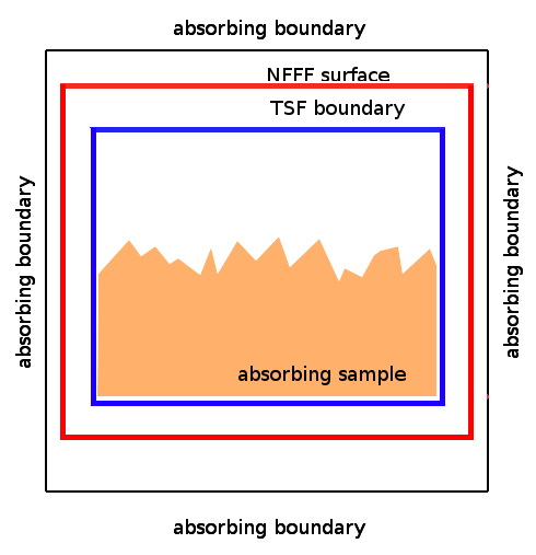
Image on the right shows a scheme of the computational volume used for the simulation (a cross-section). We use a parallelepiped
of 230x230x200 voxels bounded by simple absorbing boundary conditions. A plane wave source
is established using Total/Scattered field (TSF) approach.
A height field representing the rough surface is centred in the parallelepiped and is formed by perfect electric conductor.
To evaluate far field scattering pattern, a NFFF computational boundary is established around computational volume, just
few voxels apart the absorbing boundary conditions.
|
 |
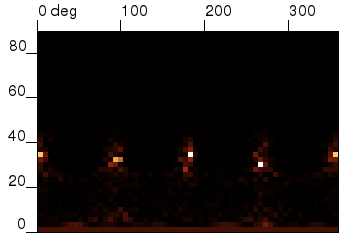
Far field radiation pattern is evaluated on a part of sphere
with prescribed radius like in transmission grating example.
A typical snapshot from the simulation is shown in the following image, showing electric field amplitude on a cross-section of
the computational volume.
As a
result we obtain a far field radiation pattern as shown below. We can see that roughness leads to scattering,
which is obvious. The results can be directly compared to e.g. far field measurements using scatterometry when we have
such measurement for particular surface. It is however necessary to perform simulation on statistically relevant surface,
e.g. on surface large enough, or average multiple simulations on different images.
As we have simulated the surface, we know in advance what should be angular position of the maxima - they should be
spaced by 90 degrees, with angle to normal of 32.5 degrees. Simulated data show the maximum at 33±2 degrees which is
in agreement to this result; with better statistics the angle uncertainty should decrease furthermore.
|