Difraction of light by a transmission grating

Summary

We will setup cubic volume with a model of single grating aperture, absorbing boundary conditions, TSF source and we will evaluate diffraction pattern produced by the grating.

What can be tested:

• periodic near-field-to-far-field transformation area
• periodic boundary conditions

Setup all this with XSvit

Note that some of the screenshots might be from an older version of XSvit.

Start the XSvit application and setup the computational volume in this way:

• Computational volume size 120x120x120 voxels, discretisation 3e-8, 3e-8, 3e-8 meters.
• 1200 computation steps
• Liao boundary conditions everywhere and periodic boundary conditions in x and y direction spanning from 10 to 110 like shown here:
  
• TSF source spanning from 10 to 110 in every direction, with orientation angles (theta, phi and psi) set to zero, sine wave with amplitude 1 V, wavelength 500 nm. Set skipping i0, in j0 and jn boundary (we don't need them as we have periodic BCs in this direction).
• Ey image outputs in every normal direction, at center of the computational volume to see the calculation progress

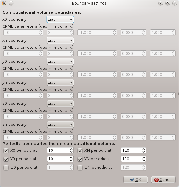
We refer to basic appplication use example for details how to adjust all these settings. Then we save the parameter file if we haven't done it before.

We will add simple model of a rectangular aperture now to the model. We will make an opaque screen and then a hole in it by writing

then we save it. Note that material objects are interpreted successively, so first we did a PEC object spanning over all the periodic volume and then we did an object with vacuum material conditions that cut part of it. Then we can save the material file using menu entry File->Save material file as... and we add the file to media entries in parameter list (by clicking on any of the Media items).

Then we can add the periodic NFFF output by Edit->Add periodic NFFF area... which calls the following dialogue: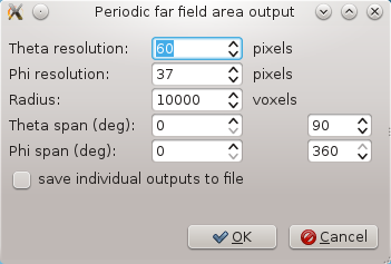

Here we set the voxel radius of the evaluated area to some very large value and we set the angular span of the area to cover whole halfspace below the aperture. Then we set parameters of the integration boundary, like this: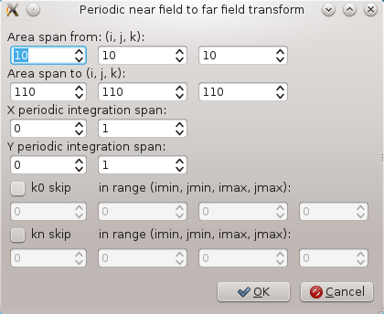

This means that for the beginning we won't use the periodic integration, only the area on the TSF boundary that is really calculated, that's why the integration spans from 0 to 1 in both x and y direction.

After setting all this the complete setup should look like this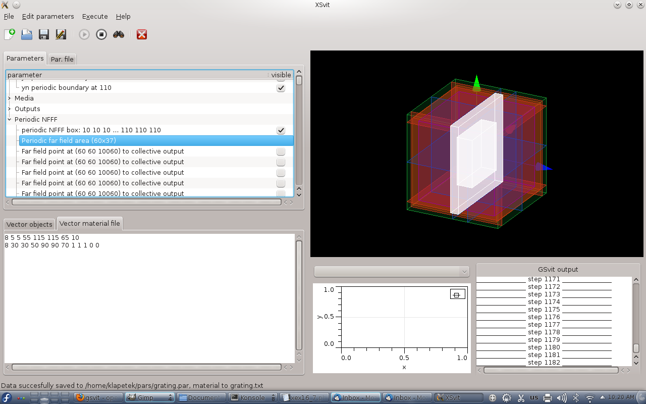

Then we can run the computation. As a result we get not only plane outputs but also a plot of total far field scattering in the directions defined by our periodic NFFF area. Now this covers whole half-space so it should look like this:

As there was no periodicity in NFFF integration this result is close to what we would get as single aperture diffaction (not exactly as for this we would not use periodic boundary conditions).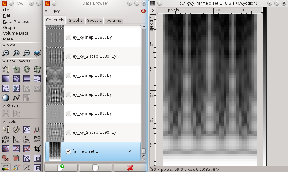

We can increase resolution of the far field area (which affects speed a lot) or zoom somewhere if we want more detailed data.

Next step is to calculate data from a periodic grating. Field is already periodic due to boundary conditions, but the far field integration is not. Ideally we would integrate over an infinite grating, but this would take infinitely long, and as you will see even quite small periodicity span takes quite long in present version of GSvit. We will change the periodicity of NFFF from 0..1 to -1..2 in both directions, which means that we will integrate over grid of 3x3 apertures. This leads to this result: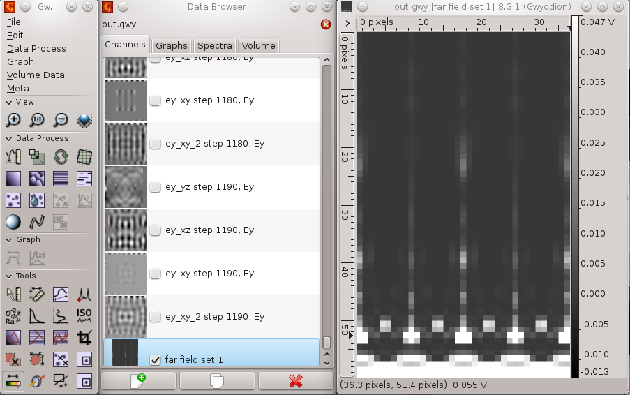

The result is here not shown in logscale like previous one was, however if you compare either normal scale or logscale view you can see thai it got changed towards analytical solution for 3x3 grating. Again note that we were using periodic field (inifinitely) so combining this with such small periodicity in integration is not correct, however in many cases it is quite close to analytical solution. With larger span of periodic integration it gets better. It is also important to use enough long pulse signal and enough computation steps, so both these parameters should be larger for more accurate results. See application example for transmission grating for some more details.

Here you can also download sample parameter file and material file.

Next example

Back to the documentation.