
|
News Features Documentation Download Participate |
Difraction of light by a reflection gratingSummaryWe will setup cubic volume with a Gwyddion height field based reflection grating pit model, absorbing boundary conditions, TSF source and we will evaluate diffraction from the grating. What can be tested:
Setup all this with XSvitNote that some of the screenshots might be from an older version of XSvit. Start the XSvit application and setup the computational volume in this way:
We refer to basic appplication use example for details how to adjust all these settings. Most of the above settings are done in the same way like in the transmission grating example. Then we save the parameter file if we haven't done it before. Now we want to load Gwyddion height field data. In this version of XSvit there is no 3D visualisation of Gwyddion data implemented yet, so we need to play with the output a bit to get the appropriate positioning of the data. First of all our data that we want to place to the center of the computational volume look like this if plotted in false color scale: 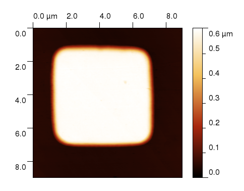
Note that the pit image is inversed in z direction to get the right result. We will add this data to the computational volume and we will cut it at each side by a thin layer of vacuum to prevent some strange effects at the border (as we have periodic BCs inside, this does not affect anything). 22 dirascaled_negative.gwy 4 -1 -1 -1 45 0 0 0 12 108 0 0 0 340 13 100 0 1 1 0 0 8 0 0 0 13 340 100 0 1 1 0 0 8 327 0 0 340 340 100 0 1 1 0 0 8 0 327 0 340 340 100 0 1 1 0 0 then we save it. Note that material objects are interpreted successively, so first we did a PEC object spanning over all the periodic volume and then we cut some parts of it. Then we can save the material file using menu entry File->Save material file as... and we add the file to media entries in parameter list (by clicking on any of the Media items). As you can see, Gwyddion data are not visualised in 3D view in this version of XSvit, so for positioning your data you need to check the computation outputs. This will be corrected in the next version. Here we at least repeat the details on how the data should be placed (as listed in computational core documentation):
Gwyddion height field is provided in Gwyddion format, and set in the material file by the following parameters are given after entity type (22), preceding material type and material parameters: filename channel mask i j k xoffset yoffset zoffset depthParameter filename corresponds to .gwy file that will be loaded (corresponding channel - if you have only one height field in your file and you haven't done some complex data processing it is probably the channel 0). If parameter mask is 1, only data under mask are used for this purposes (see Gwyddion documentation to see what a mask is). If parameter mask is -1, the inverse of mask is used. Note that real Gwyddion datafield dimensions are used to scale the datafield within the computational space. Vector (i j k) in voxel coordinates defines the relative coordinate center in computation space and direction. (e.g. -1 -1 10 means that the field will be oriented in z normal and its zero coordinate will be shifted by 10 voxels in z). Parameters xoffset, yoffset and zoffset are in dfield physical coordinates and are used to further shift the dfield if necessary. If these are zero, top left corner is aligned. Parameter depth (in voxels) defines the depth to which the material is assigned (with same orientation as the axis). Then we can add the periodic NFFF output by Edit->Add periodic NFFF area.... We will set this with resolution of 90 in theta and 1 in phi, spanning from 170 to 180 in theta and from 90 to 91 in phi. This means that we want only single row of far field points; the result will be shown in Gwyddion output file as a graph. Finally we setup the periodic NFFF integration boundary. It will span to 15..325 for x and y and 15..60 for z, skipping kn boundary (as this is inside PEC so it would add nothing to the far field data). We will integrate periodically in range of -2..3 for both directions, which means that we will use 5x5 repetitions of the field above our pit. 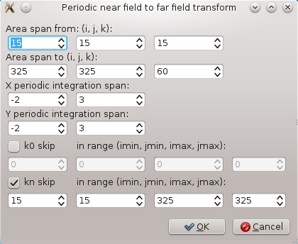
After setting all this the complete setup should look like this 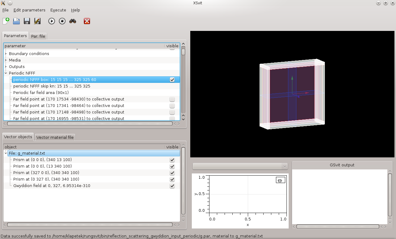
Then we can save all files and run the computation. This might take quite long as we have larger computational volume than in previous examples, and also much more more computation steps. As a result we get graph of diffraction within 0-10 degrees from normal where we can see several diffraction maxima. 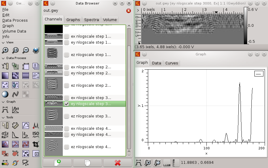
Here you can also download sample data for this example. (c) Petr Klapetek, 2013 |